
This article at OpenGenus will examine the notion of Hinge loss for SVM, providing insight into loss function.
Table of Contents:
- Introduction
- The Hinge Loss Function
- Soft Margin Classification
- The Regularization Parameter
- Code for Hinge Loss for SVM
- Advantages and disadvantages of Hinge loss for SVM
- Comparison between Loss Functions
- Conclusion
Introduction
Support Vector Machines (SVMs) are a powerful class of supervised machine learning algorithms that can be used for both classification and regression tasks. SVMs are particularly useful for solving classification problems where the data points are not linearly separable. SVMs have been successfully applied in a wide range of fields, including image classification, natural language processing, and bioinformatics.
SVMs work by finding a hyperplane that best separates the classes in the input data. However, in many real-world scenarios, the data is not linearly separable, meaning that a hyperplane cannot perfectly separate the classes. In such cases, SVMs use a technique called soft margin classification, which allows for some misclassification of data points. To achieve this, SVMs use a loss function called the hinge loss.
In this article, we will explore hinge loss in more detail and explain how it works in the context of SVMs.
The Hinge Loss Function
The hinge loss function is a type of loss function that is used to penalize the SVM for misclassifying data points. The loss function is defined as:
L(y, f(x)) = max(0, 1 - y*f(x))
where y is the true class label (y = -1 or y = 1) and f(x) is the predicted score for the positive class. If yf(x) >= 1, then the loss is zero, which means that the prediction is correct. If yf(x) < 1, then the loss is proportional to the distance from the correct prediction.
Here's a plot of the Hinge Loss:
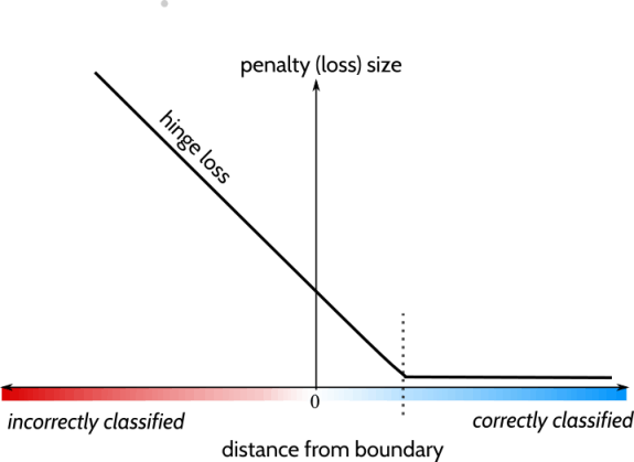
The hinge loss function is essentially a "hinged" or piecewise-linear function that has a slope of -1 when the predicted label is correct, and a slope of 0 when the predicted label is incorrect but within the margin. When the predicted label is incorrect and outside the margin, the hinge loss function has a slope of 1.
Sample calculation:
Suppose we have a binary classification problem with two classes (y = -1 or y = 1) and our model predicts the following scores for three examples:
Example 1: f(x) = 0.8
Example 2: f(x) = -0.4
Example 3: f(x) = 1.2
Assuming that the true labels are:
Example 1: y = 1
Example 2: y = -1
Example 3: y = 1
We can calculate the Hinge Loss for each example as follows:
Example 1: L(y, f(x)) = max(0, 1 - yf(x)) = max(0, 1 - 10.8) = 0.2
Example 2: L(y, f(x)) = max(0, 1 - yf(x)) = max(0, 1 - (-1)(-0.4)) = 0.6
Example 3: L(y, f(x)) = max(0, 1 - yf(x)) = max(0, 1 - 11.2) = 0
As we can see, the Hinge Loss is zero for Example 3, which means that the prediction is correct. The Hinge Loss for Example 1 is smaller than the Hinge Loss for Example 2, which indicates that the model is more confident in its prediction for Example 1.
Soft Margin Classification
The soft margin classification technique used by SVMs involves minimizing the hinge loss function subject to a constraint that limits the magnitude of the weight vector. This constraint is known as the regularization parameter, and it determines the trade-off between achieving a low hinge loss and having a small weight vector. The regularization parameter is typically set using cross-validation techniques.
The soft margin classification technique is based on the idea of allowing some misclassification of data points in order to find a more generalizable solution. The margin is defined as the distance between the hyperplane and the closest data point from either class. The goal of SVMs is to find the hyperplane that maximizes the margin between the two classes.
However, when the data points are not linearly separable, the SVM cannot find a hyperplane that perfectly separates the classes. In this case, the SVM introduces a slack variable that allows for some misclassification of data points. The slack variable represents the distance between a misclassified data point and the correct side of the margin. The soft margin classification technique tries to minimize the sum of the hinge loss function and the slack variable subject to the regularization parameter.
The Regularization Parameter
The regularization parameter, often denoted as C, is a hyperparameter that determines the trade-off between achieving a low hinge loss and having a small weight vector. A small value of C corresponds to a large margin and a high tolerance for misclassification, while a large value of C corresponds to a narrow margin and a low tolerance for misclassification.
If C is set to a very large value, then the SVM will try to minimize the hinge loss function at all costs, even if it means overfitting the data. Conversely, if C is set to a very small value, then the SVM will prioritize having a large margin, even if it means misclassifying some data points. The regularization parameter is typically set using cross-validation techniques to find the optimal value that balances the trade-off.
Code for Hinge Loss for SVM
Here's an example implementation of hinge loss for SVM in Python:
import numpy as np

def hinge_loss(y_true, y_pred):
    loss = np.maximum(0, 1 - y_true * y_pred)
    return np.mean(loss)

def svm_loss(X, y, W, reg):
    num_classes = W.shape[1]
    num_train = X.shape[0]
    scores = X.dot(W)
    correct_class_scores = scores[np.arange(num_train), y]
    margins = np.maximum(0, scores - correct_class_scores[:, np.newaxis] + 1)
    margins[np.arange(num_train), y] = 0
    loss = np.sum(margins) / num_train
    loss += 0.5 * reg * np.sum(W * W)
    return loss
In this code, hinge_loss() computes the hinge loss for a single data point, given its true label y_true and predicted label y_pred. svm_loss() computes the overall SVM loss for a given set of data X and labels y, weight matrix W, and regularization strength reg.
The code first computes the scores for each class for each data point using the dot product of the input data and the weight matrix. It then computes the correct class scores and the margins for each incorrect class. The loss is then computed as the mean of the maximum between 0 and the margins, plus a regularization term.
This implementation assumes that the labels y are encoded as integers ranging from 0 to num_classes-1. The svm_loss() function also assumes that the weight matrix W has already been initialized and has the correct shape for the given input data.
This is just one example implementation of hinge loss for SVM, and there are many variations and optimizations that can be made depending on the specific application and requirements.
Advantages and disadvantages of Hinge loss for SVM
- Advantages:
-
Margin maximization: Hinge loss is designed to maximize the margin between different classes, which is the distance between the separating hyperplane and the closest data points. Maximizing the margin can lead to better generalization performance and improve the ability of the classifier to handle new data.
-
Robustness to outliers: Hinge loss is less sensitive to outliers than other loss functions like mean squared error. Outliers can have a significant impact on the learned model and can cause overfitting, but hinge loss mitigates this effect by ignoring points that are correctly classified but are still close to the decision boundary.
-
Sparsity: SVM with hinge loss can result in a sparse model, which means that many of the coefficients in the weight vector are set to zero. This can make the model more interpretable and reduce the computational cost of inference.
- Disadvantages:
-
Non-smoothness: The hinge loss function is non-smooth and non-differentiable at 0, which can make it difficult to optimize using some numerical optimization methods. However, sub-gradient methods can be used to optimize the hinge loss function.
-
Parameter sensitivity: SVM with hinge loss has a regularization parameter that controls the trade-off between maximizing the margin and minimizing the classification error. The choice of this parameter can have a significant impact on the performance of the model, and selecting the optimal value can be challenging.
-
Limited applicability: SVM with hinge loss is a binary classifier and cannot be directly applied to multi-class problems. However, there are techniques, such as one-vs-rest or one-vs-one, that can be used to extend SVM with hinge loss to multi-class problems.
Overall, hinge loss for SVM is a popular and effective method for binary classification tasks, particularly in scenarios where there are a large number of features and the data is high-dimensional. However, it may not be suitable for all types of data and may require careful parameter tuning to achieve good performance.
Comparison between Loss Functions
There are several loss functions used in machine learning for classification tasks, including the Hinge Loss, Cross Entropy Loss, Logistic Loss (also known as Sigmoid Loss), and Log Loss (also known as Binary Cross Entropy Loss). Here's a comparison of these loss functions:
- Hinge Loss:
- Used in SVMs and related models for binary classification tasks.
- Penalizes incorrect predictions proportional to the distance from the decision boundary.
- Does not produce probabilistic outputs.
- Cross Entropy Loss:
- Used in neural networks and other models for multi-class classification tasks.
- Measures the difference between the predicted probability distribution and the true distribution.
- Produces probabilistic outputs.
- Logistic Loss (Sigmoid Loss):
- Used in logistic regression and related models for binary classification tasks.
- Measures the difference between the predicted probability and the true label.
- Produces probabilistic outputs.
- Log Loss (Binary Cross Entropy Loss):
- Similar to the Cross Entropy Loss, but used for binary classification tasks.
- Measures the difference between the predicted probability and the true label.
- Produces probabilistic outputs.
The Hinge Loss is commonly used in SVMs because it is well-suited for models that rely on maximizing the margin between the decision boundary and the data points. Other loss functions like the Cross Entropy Loss and Logistic Loss are not used in SVMs because they are not designed to maximize the margin. Additionally, these loss functions produce probabilistic outputs, which is not required in SVMs.
In summary, the choice of loss function depends on the model and the task at hand. The Hinge Loss is a good choice for SVMs and related models, while other loss functions like the Cross Entropy Loss and Logistic Loss are better suited for neural networks and logistic regression models.
Conclusion
To conclude this article at OpenGenus, hinge loss is a commonly used loss function for training support vector machines (SVM) in binary classification tasks. The hinge loss function encourages the SVM to maximize the margin between the decision boundary and the closest data points, while penalizing points that are misclassified or lie within the margin. The advantages of hinge loss for SVM include margin maximization, robustness to outliers, and sparsity of the resulting model. However, hinge loss is non-smooth and non-differentiable, which can make it difficult to optimize using some numerical optimization methods, and the choice of regularization parameter can have a significant impact on the performance of the model. Despite its limitations, hinge loss for SVM is a powerful tool for binary classification tasks in high-dimensional data, and is widely used in applications such as image classification, natural language processing, and bioinformatics.