
Get this book -> Problems on Array: For Interviews and Competitive Programming
Flow networks are fundamentally directed graphs, where edge has a flow capacity consisting of a source vertex and a sink vertex. The aim of the max flow problem is to calculate the maximum amount of flow that can reach the sink vertex from the source vertex keeping the flow capacities of edges in consideration. The flow at each vertex follows the law of conservation, that is, the amount of flow entering the vertex is equal to the amount of flow leaving the vertex, except for the source and the sink. The entire amount of flow leaving the source, enters the sink.
For example-
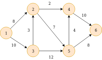
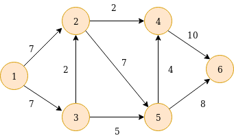
The source vertex is 1 and 6 is the sink. The above graph indicates the capacities of each edge. The maximum flow possible in the the above network is 14. A possible flow through each edge can be as follows-
Some important terms
1. Residual Capacity and Residual Graph
The residual capacity of an edge is equal to the original flow capacity of an edge minus the current flow. The graph with edge capacities equal to the corresponding residual capacities is called a residual graph.
2. Augmenting Path
Augmenting path is a path in the flow network where the start vertex is the source and the destination vertex is the sink.
3. Cut and Cut-Set
A cut in a graph G=(V,E) is defined as C=(S,T) where S and T are two disjoint subsets of the V. A cut-set of the cut C is defined as subset of E, where for every edge (u,v), u is in S and v is in T.
4. Level Graph
In level graph we assign a level to each node, which is equal to the shortest distance of the source to the node.
5. Minimum cut
It is the the minimum total weight of the edges, which after removal would disconnect the source from the sink.
Algorithms for calculating maximum flow
1. Ford Fulkerson Algorithm
The Ford Fulkerson Algorithm picks each augmenting path(chosen at random) and calculates the amount of flow that travels through the path. This flow is equal to the minimum of the residual capacities of the edges that the path consists of.
The time complexity for the algorithm is O(MaxFlow.E). In the worst case, the time complexity can go to O(EV3).
2. Edmond Karp Implementation
The Edmond Karp Implementation is a variation of the Ford Fulkerson Algortihm. In this implementation we use BFS and hence end up choosing the path with minimum number of edges. The worst case time complexity in this case can be reduced to O(VE2).
3. Dinic's Algorithm
Dinic's Algorithm is implemented using BFS by creating a level graph from the residual graph. We start by assigning levels to each of the nodes using BFS. Each path chosen should consist of all the levels from 0 to n, where the source has level 0, and the sink has level n. The above procedure is repeated on the obtained residual graphs. The max flow is determined when there is no path left from the source to sink. This is known as Dinic's Blocking Flow Algorithm.
The time complexity of the algorithm is O(EV2) where E and V are the number of edges and vertices respectively.
This Algorithm was furthur optimized by using Dynamic Trees, which led to the reduction of the time complexity to O(VElogV).
4. Push Relabel Algorithm
Push Relabel algorithm is more efficient that Ford-Fulkerson algorithm.
It considers one vertex at a time instead of looking at the entire network at once. Each vertex has an excess flow value and height value associated with it. A vertex can push to an adjacent vertex with lower height. Excess flow is the difference between total incoming flow and total outgoing flow of the vertex. Once a node has excess flow, it pushes flow to a smaller height node. If water gets locally trapped at a vertex, the vertex is Relabeled (its height is increased).
The algorithm considers every vertex and checks if it has an excess flow, if it does then it tries to perform either a push or a relabel on it. At the end we get all the vertices with zero excess flow except source and sink.
The time complexity of the algorithm is O(EV2) where E and V are the number of edges and vertices respectively.
5. Orlin's Algorithm
This algorithm is efficient in determining maximum flow in sparce graphs.
The algorithm searches for the shortest augmenting path in the residual network of the graph iteratively. During the iterations,if the distance label of a node becomes greater or equal to the number of nodes, then no more augmenting paths can exist in the residual network. This condition terminates the algorithm.
The time complexity of the algorithm is O(EV) where E and V are the number of edges and vertices respectively.
Applications of the Max Flow Problem
1. Finding vertex-disjoint paths : The Max flow problem is popularly used to find vertex dijoint paths. The algorihtm proceeds by splitting each vertex into incoming and outgoing vertex, which are connected by an edge of unit flow capacity while the other edges are assigned an infinite capacity. The max flow from the source to sink now denotes the no. of vertex disjoint paths. Since every vertex allows only unit capacity, it has only one path passing through it.
2. Flows with multiple sources and multiple sinks: In this scenario, all the source vertices are connected to a new source with edges of infinite capacity. Same is done for the sink vertices. The max flow can now be calculated by the usual methods of this new graph made by the above constructions.
3. Bipartite matching problem: A bipartite matching is a set of the edges chosen from a bipartite graph, such that no two edges have a common endpoint. The bipartite graph is converted to a flow network by adding source and sink. It is claimed that the value of the maximum flow in the flow network is the size of the maximum bipartite matching in the bipartite graph.
4. Airline scheduling: Every flight has 4 parameters, departure airport,
destination airport, departure time, and arrival time. We can use a single airplane for flight A and B if, either the destination of A is departure of B and there is enough time between arrival time of A and departure time of B for maintenance, or there is a flight that takes the airplane from the destination of A to departure B with enough time for maintenance. Aim is to schedule n flights using at most k planes. A graph is made such that we have an edge from A to B if the same plane can serve both the flights.
The solution is as follows: there is a way to schedule all the flights using at most k planes if and only if there is a feasible circulation in the network.
5. Image segmentation: This is done by converting the image into a flow graph, where every pixel is a vertex and which connects neighboring pixel-vertices in a 4-neighboring system. There are 2 more vertices, that are the source and sink. Then a max-flow algorithm is run on the graph in order to find the minimum cut, which produces the optimal segmentation.
Question
How are augmenting paths chosen in the original Ford Fulkerson Algorithm?
With this article at OpenGenus, you must have a good understanding of Overview of Maximum Flow Problem which includes algorithms, terms, applications and much more. Enjoy.