
In this article we will briefly discuss about the travelling salesman problem and the branch and bound method to solve the same.
What is the problem statement ?
Travelling Salesman Problem is based on a real life scenario, where a salesman from a company has to start from his own city and visit all the assigned cities exactly once and return to his home till the end of the day. The exact problem statement goes like this,
"Given a set of cities and distance between every pair of cities, the problem is to find the shortest possible route that visits every city exactly once and returns to the starting point."
There are two important things to be cleared about in this problem statement,
- Visit every city exactly once
- Cover the shortest path
What is branch and bound ?
Before going into the details of the branch and bound method lets focus on some important terms for the same,
-
State Space Search Method - Remember the word sample space from the probability theory ? That was a set of all the possible sample outputs. In a similar way,state space means, a set of states that a problem can be in. The set of states forms a graph where two states are connected if there is an operation that can be performed to transform the first state into the second.
In a lighter note, this is just a set of some objects, which has some properties/characteristics, like in this problem, we have a node, it has a cost associated to it. The entire state space can be represented as a tree known as state space tree, which has the root and the leaves as per the normal tree, which are interms the elements of the statespace having the given graph node and a cost associated to it. -
E-node - Expanded node or E node is the node which is been expanded. As we know a tree can be expanded using both BFS(Bredth First Search) and DFS(Depth First Search),all the expanded nodes are known as E-nodes.
-
Live-node - A node which has been generated and all of whose children are not yet been expanded is called a live-node.
-
Dead-node - If a node can't be expanded further, it's known as a dead-node.
The word, Branch and Bound refers to all the state space search methods in which we generate the childern of all the expanded nodes, before making any live node as an expanded one. In this method, we find the most promising node and expand it. The term promising node means, choosing a node that can expand and give us an optimal solution. We start from the root and expand the tree untill unless we approach an optilmal (minimum cost in case of this problem) solution.
How to get the cost for each node in the state space tree ?
To get further in branch and bound, we need to find the cost at the nodes at first. The cost is found by using cost matrix reduction, in accordance with two accompanying steps row reduction & column reduction.
In general to get the optimal(lower bound in this problem) cost starting from the node, we reduce each row and column in such a way that there must be atleast one 0 in each row and column. For doing this, we just need to reduce the minimum value from each row and column.
For example, suppose we have a cost matrix as shown below,
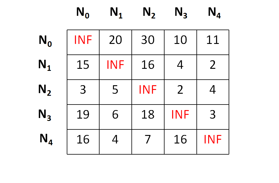
Let's start from node N0,;lets consider N0 as our first live node.
First of all we will perform the row operations and to do the same, we need to subtract the minimum value in each row from each element in that row. The minimums and the row reduced matrix is shown below,
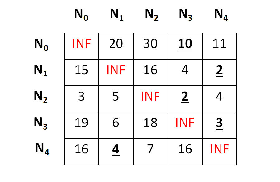
And after row reduction,
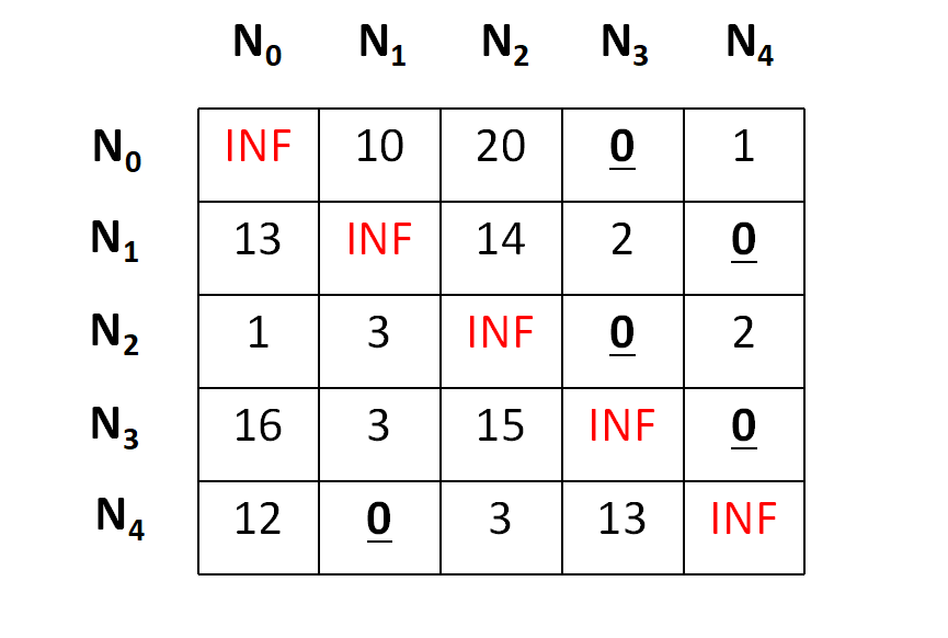
Now we need to perform the column operation in the same manner and we will get a final matrix as below,
The total cost at any node is calculated by making a sum of all reductions, hence the cost for the node N0 can be depicted as,
cost = 10 + 2 + 2 + 3 + 4 + 1 + 3 = 25
Now as we have founded the cost for the root node, it's the time for the expansion, and to do so, we have four more nodes namely, N1,N2,N3,N4.
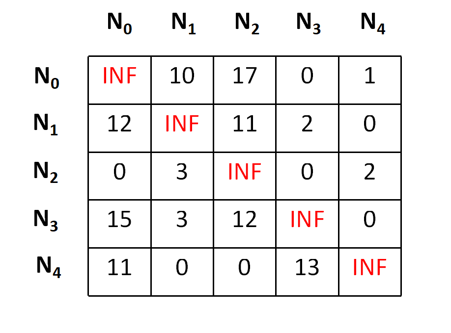
Let's add the edge from N0 to N1 in our search space. To do so, we need to set outgoing routes for city N0 to INF as well as all incoming routes to city N1 to INF.Also we will set the (N0,N1) position of the cost matrix as INF. By doing so, we are just focusing on the cost of the node N1, that's an E-node. In an easier note, we have just forgotten that the graph has a N0 node, but we are focusing on something that the graph has been started from the N1 node. Following the transformation we have something as below,
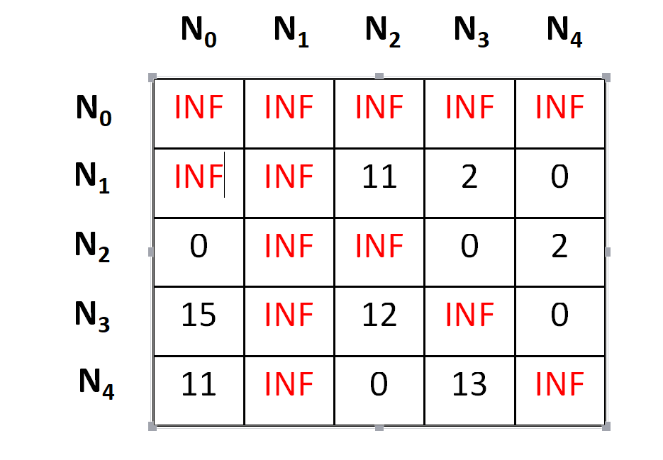
Now it's the time to repeat the lower bound finding(row-reduction and the column-reduction) part that we have performed earlier as well, following which we will get that the matrix is already in reduced form, i.e. all rows and all columns have zero value.
Now it's the time to calculate the cost.
cost = cost of node N0 + cost of the (N0,N1) position(before setting INF) + lower bound of the path starting at N1 = 25 + 10 + 0 = 35
Hence the cost for the E-Node N1 is 35.
In a similar way we can find that,
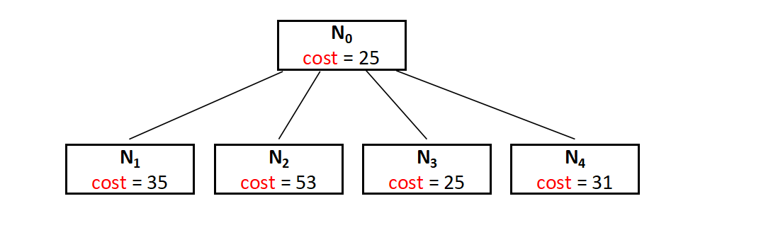
For N2 the cost is 53,
For N3 the cost is 25,
And for N4 the cost is 31.
Now we have a part of state space tree ready, whcih can be shown as below,
How to get towards the optimal solution ?
To get the optimal solution, we have to choose the next live node from the list of the extended nodes (E-nodes) and repeat the same procedure of extending the tree further by calculating the lower bound.
Here in the partially built space search tree above we have the Node N3 as the node having the minimum cost and we can consider it as the live node and extend the tree further. This step is repeated until unless we find a dead node and can not extend the tree further. The cost of the dead node (leaf node) will be the answer.
The entire space search tree can be drawn as follow,
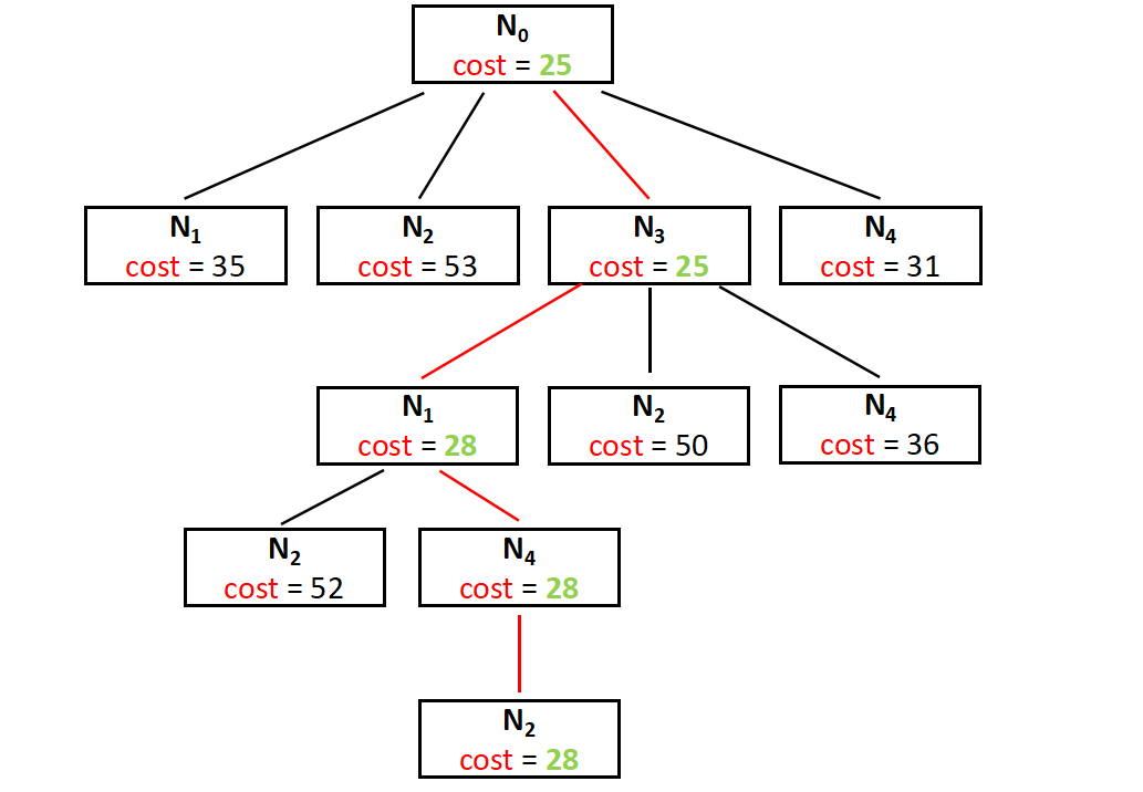
And the final cost is 28, that's the minimum cost for a salesman to start from N0 and return to N0 by covering all the cities.
The Main Code
Now after knowing the entire process, this thing is easier to code. We have tried something new this time by attaching some more datastructures and objects to print the path as well. Have a look at the following code in order to understand it,
#include <bits/stdc++.h>
using namespace std;

// number of total nodes
#define N 5
#define INF INT_MAX

class Node
{
public:
    vector<pair<int, int>> path;
    int matrix_reduced[N][N];
    int cost;
    int vertex;
    int level;
};

Node* newNode(int matrix_parent[N][N], vector<pair<int, int>> const &path,int level, int i, int j)
{
    Node* node = new Node;
    node->path = path;
    if (level != 0)
        node->path.push_back(make_pair(i, j));
    memcpy(node->matrix_reduced, matrix_parent,
        sizeof node->matrix_reduced);
    for (int k = 0; level != 0 && k < N; k++)
    {
        node->matrix_reduced[i][k] = INF;
        node->matrix_reduced[k][j] = INF;
    }

    node->matrix_reduced[j][0] = INF;
    node->level = level;
    node->vertex = j;
    return node;
}

void reduce_row(int matrix_reduced[N][N], int row[N])
{
    fill_n(row, N, INF);

    for (int i = 0; i < N; i++)
        for (int j = 0; j < N; j++)
            if (matrix_reduced[i][j] < row[i])
                row[i] = matrix_reduced[i][j];

    for (int i = 0; i < N; i++)
        for (int j = 0; j < N; j++)
            if (matrix_reduced[i][j] != INF && row[i] != INF)
                matrix_reduced[i][j] -= row[i];
}

void reduce_column(int matrix_reduced[N][N], int col[N])
{
    fill_n(col, N, INF);

    for (int i = 0; i < N; i++)
        for (int j = 0; j < N; j++)
            if (matrix_reduced[i][j] < col[j])
                col[j] = matrix_reduced[i][j];

    for (int i = 0; i < N; i++)
        for (int j = 0; j < N; j++)
            if (matrix_reduced[i][j] != INF && col[j] != INF)
                matrix_reduced[i][j] -= col[j];
}

int cost_calculation(int matrix_reduced[N][N])
{
    int cost = 0;

    int row[N];
    reduce_row(matrix_reduced, row);

    int col[N];
    reduce_column(matrix_reduced, col);

    for (int i = 0; i < N; i++)
        cost += (row[i] != INT_MAX) ? row[i] : 0,
            cost += (col[i] != INT_MAX) ? col[i] : 0;

    return cost;
}

void printPath(vector<pair<int, int>> const &list)
{
    for (int i = 0; i < list.size(); i++)
        cout << list[i].first + 1 << " -> "
             << list[i].second + 1 << endl;
}

class comp {
public:
    bool operator()(const Node* lhs, const Node* rhs) const
    {
        return lhs->cost > rhs->cost;
    }
};

int solve(int adjacensyMatrix[N][N])
{
    priority_queue<Node*, std::vector<Node*>, comp> pq;
    vector<pair<int, int>> v;
    Node* root = newNode(adjacensyMatrix, v, 0, -1, 0);
    root->cost = cost_calculation(root->matrix_reduced);
    pq.push(root);
    while (!pq.empty())
    {
        Node* min = pq.top();
        pq.pop();
        int i = min->vertex;
        if (min->level == N - 1)
        {
            min->path.push_back(make_pair(i, 0));
            printPath(min->path);
            return min->cost;
        }

        for (int j = 0; j < N; j++)
        {
            if (min->matrix_reduced[i][j] != INF)
            {
                Node* child = newNode(min->matrix_reduced, min->path,
                    min->level + 1, i, j);

                child->cost = min->cost + min->matrix_reduced[i][j]
                            + cost_calculation(child->matrix_reduced);

                pq.push(child);
            }
        }

        delete min;
    }
}

int main()
{
    int adjacensyMatrix[N][N] =
    {
        { INF, 20, 30, 10, 11 },
        { 15,  INF, 16,  4,  2 },
        { 3,   5,  INF, 2,  4 },
        { 19,   6,   18,   INF, 3 },
        { 16,   4,   7,   16, INF }
    };

    cout << "\nCost is " << solve(adjacensyMatrix);

    return 0;
}
Code Explanation :
We would briefly go through the three main functions of the algorithm and try to understand how the algorithm is working, which is pretty similar to what we have learbed above.
reduce_row()
As the name suggests, this function is used to reduce the desired row. In this function we are using an awesome builtin function namely fill_n() available in the C++ STL.
Have a look at the syntax,
void fill_n(iterator begin, int n, type value);
This function makes it easy to fill an entire row with the desired value(INF here).
Now it's time to run two loops, one for the minimum value finding for each row and one for making the reduction. Have a look at the below snippet of the code.
/// row[i] is the minimum value for the ith row
for (int i = 0; i < N; i++)
        for (int j = 0; j < N; j++)
            if (matrix_reduced[i][j] < row[i])
                row[i] = matrix_reduced[i][j];

/// subtracting the minimum value and reducing the matrix
for (int i = 0; i < N; i++)
    for (int j = 0; j < N; j++)
        if (matrix_reduced[i][j] != INF && row[i] != INF)
            matrix_reduced[i][j] -= row[i];
You may guess the run time complexity of the above function is O(n^2) because the loop has two iterations embeded one inside the other.
The run time complexity of the fill_n() function is Linear, i.e O(n).
reduce_column()
As the name suggests, this function is used to reduce the desired column, in a similar fashion to what we have done above.
This function makes it easy to fill an entire column with the desired value(INF here).
Now it's time to run two loops, one for the minimum value finding for each row and one for making the reduction. Have a look at the below snippet of the code.
fill_n(col, N, INF);

/// row[i] is the minimum value for the ith row
for (int i = 0; i < N; i++)
    for (int j = 0; j < N; j++)
        if (matrix_reduced[i][j] < col[j])
            col[j] = matrix_reduced[i][j];

///for reducing the matrix
for (int i = 0; i < N; i++)
    for (int j = 0; j < N; j++)
        if (matrix_reduced[i][j] != INF && col[j] != INF)
            matrix_reduced[i][j] -= col[j];
You may guess the run time complexity of the above function is O(n^2) because the loop has two iterations embeded one inside the other.
The run time complexity of the fill_n() function is Linear, i.e O(n).
cost_calculation()
This function need to get the reduced matrix as a parameter, perform the row reduction, the column reduction successively and then calculate the cost.
This can been seen below.
int cost_calculation(int matrix_reduced[N][N])
{
    /// setting the initial cost as 0
    int cost = 0;

    /// reducing the row
    int row[N];
    reduce_row(matrix_reduced, row);

    /// reducing the column
    int col[N];
    reduce_column(matrix_reduced, col);

    /// main cost calculation
    for (int i = 0; i < N; i++)
        cost += (row[i] != INT_MAX) ? row[i] : 0,
            cost += (col[i] != INT_MAX) ? col[i] : 0;

    return cost;
}
The time complexity of the program is O(n^2) as explained above for the row and column reduction functions.
What is the final time complexity ?
Now this thing is tricky and need a deeper understanding of what we are doing. We are actually creating all the possible extenstions of E-nodes in terms of tree nodes. Which is nothing but a permutation. Suppose we have N cities, then we need to generate all the permutations of the (N-1) cities, excluding the root city. Hence the time complexity for generating the permutation is O((n-1)!), which is equal to O(2^(n-1)).
Hence the final time complexity of the algorithm can be O(n^2 * 2^n).