In this article, we will learn Why is Dimensionality Reduction important and 5 different Types of Dimensionality Reduction Techniques like Principal Component Analysis, Missing Value Ratio, Random Forest, Backward Elimination and Forward Selection.

Table of Contents:

1. Introduction
2. What is Dimensionality?
3. What is Dimensionality Reduction?
4. Why do we need Dimensionality Reduction?
5. Types of Dimensionality Reduction Techniques
   5.1. Principal Component Analysis
   5.2. Missing Value Ratio
   5.3. Random Forest
   5.4. Backward Elimination
   5.5. Forward Selection

Let us get started with Types of Dimensionality Reduction Techniques.

Introduction

Have you ever dealt with a dataset containing tens of thousands of features? Consider how challenging it would be to create Machine Learning Models with that many attributes and how easy it would be if we could just get rid of features that we don't need!

Before going on, lets answer the question, What is Dimensionality?

Dimensionality refers to the number of columns, input features, attributes, and variables in a dataset. For example, consider a simple Students dataset with two features: Name and Age; now, this is a 2-dimensional Dataset, if we add a third feature, such as Height, this becomes a 3-dimensional dataset.

Basically, to put it in a nutshell, the number of features in a dataset is called its dimensionality.

What is Dimensionality Reduction?

So, now as you have an understanding of what Dimensionality is, it wouldn’t take much time to guess, what Dimensionality Reduction means, yes, it means removing features from a dataset.

The reduction of input features from a dataset to ease the process is called as Dimensionality Reduction.

But wait, wouldn't removing features from our dataset have a detrimental impact on our machine learning model? Isn’t it true, as we have heard, that having a large amount of data/input feature aids in creating good predictions? Removing the features won't affect?

Now this brings us to:

Why do we need Dimensionality Reduction and it's Importance?

Till now, what we have learned is that dimensionality reduction means, reduction of input features, but no one told us what is the problem with many input features? Let’s answer that:

• Machine learning algorithms suffer from having too many input features.
• A large quantity of space is used by having too many input features.
• Too many input variables bring in the curse, i.e. curse of dimensionality.

So, what are the Advantages & Why do we need it?

• Data visualization is aided by the reduced dimensionality of dataset features.
• A lower number of dimensions in data equals less training time and computer resources, which improves machine learning algorithms' overall performance.
• Multicollinearity is addressed by deleting duplicate features.
• When there are many features in the data, the model tends to overfit, dimensionality reduction helps in avoiding the problem of overfitting

Now, since we have the understanding of What is Dimensionality, What do we mean by Dimensionality Reduction and what are the advantages of Dimensionality Reduction, let’s look at various Dimensionality Reduction Techniques.

Types of Dimensionality Techniques:

We will be covering 5 different Dimensionality Reduction Techniques:

1. Principal Component Analysis
2. Missing Value Ratio
3. Random Forest
4. Backward Elimination
5. Forward Selection

1. Principal Component Analysis:

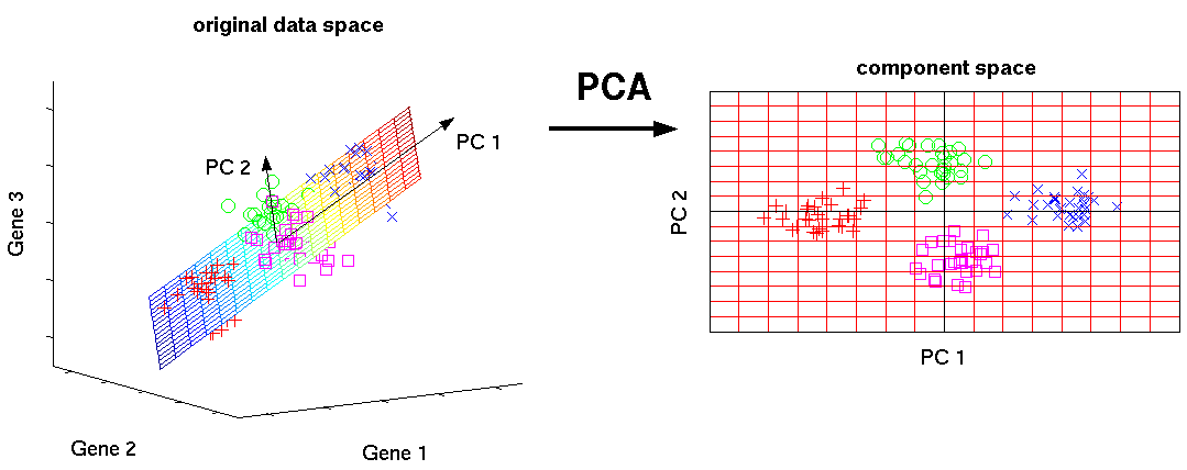
PCA is a method for extracting new variables from a large set of data. Through the use of orthogonal transformation, Principal Component Analysis turns correlated feature observations into a set of statistically independent features. These newly extracted variables/features are called Principal Component. Principal Component Analysis is a form of unsupervised Machine Learning algorithm used for dimensionality reduction.

It is always implemented on symmetric correlation or covariance matrix, this implies that the matrix is should be numerical and contain data that is standardize.

Basically, PCA is a typical approach for visualizing and pre-processing high-dimensional data. By preserving as much variance as feasible, PCA decreases the dimensionality (number of variables) of a data collection.

Some key points about Principal Component Analysis:

• A linear combination of the original variables is referred to as a principal component.
• The first principal component is extracted in such a way that it explains the most variation in the dataset.
• The second principal component, which is unrelated to the first, attempts to explain the remaining variation in the dataset.
• The third principle component attempts to explain the variation that the previous two principal components have failed to explain, and so on.

The graphic below depicts how PCA can be used to turn high-dimensional data (3 dimensions) into low-dimensional data (2 dimensions).

2. Missing Value Ratio:

The first step in creating a Machine Learning Model is to analyze the available data. What should we do if we are provided a dataset that contains a large number of missing values/data? Our ML model will suffer from missing values. So, you may either drop the column or fill in the missing data. How should we determine whether to eliminate the column or fill in the missing values? Well, that relies entirely on the relevance of the column and whether or not we will need it for our prediction. However, I use a 50 percent rule, which states that if more than half of the values are missing, the item is dropped.

Let’s understand this by an example, lets take the very famous Titanic Survival Prediction dataset.

Import pandas as pd

titanic_train = pd.read_csv(‘train.csv’)
titanic_train.head(8)

Once we call the above code the, the dataset it displayed:

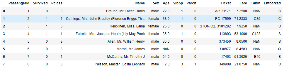
As we can see that the above dataset has 12 columns, now lets look for the missing values, we do that using, isnull() and sum().

titanic_data.isnull().sum()

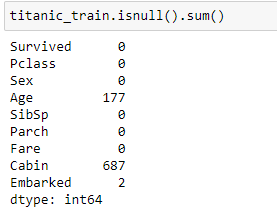
We can clearly determine that the Column Age has 177 null values, the column Cabin has 687 null values and the column Embarked has 2 null values.

Now, lets think, do we need these 3 columns for our prediction? The age column is important, but do we need the cabin column? It’s not that important plus it has 687 missing values, its will be completely fine if we drop it

titanic_train.drop(‘cabin’,axis=1)

Now, let’s work on the missing values of the Age column and the Embarked column, what we can do is fill the missing values with the mean of the Age column. This is how we do it.

titanic_train[‘Age’].mean()
titanic_train[‘Age’].fillna(titanic_train[‘Age’].mean(),inplace = True)

Now let’s fill in the missing values of the Embarked Column

titanic_data['Embarked'].fillna(titanic_data['Embarked'].mode()[0], inplace=True)

what we did is we replaced the missing values in the “Embarked” column with mode value.

Now our dataset is ready, with no missing values.

3. Random Forests

One of the most well-known and appropriate feature selection techniques is Random Forest. It's a tree-based model that's frequently used for non-linear data regression and classification. It already comes with in-built feature importance so we don’t need to program it separately. However, we must only use numeric values in this algorithm as it only takes them.

Let's use the Titanic Dataset to implement the Random Forest algorithm.

Earlier we dealt with the missing values, now, lets deal with non-numeric values before we shift to implementing Random Forests.

Let’s look at the dataset once more.

Before going ahead, let’s make it clear that the Name, Ticket, Fare, Cabin columns are of no use to us in making the prediction.

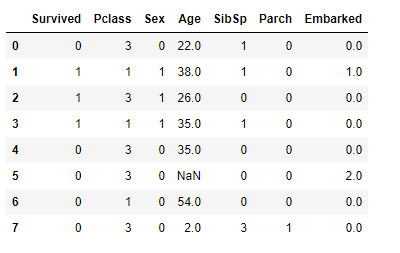
As we can see that the Sex and the Embarked Columns are of non-numeric types. Let’s convert them into numeric values. We will replace male by 0 and female by 1 in the sex column and for the Embarked column we will replace the S by 0, C by 1 and Q by 2.

titanic_data.replace({'Sex':{'male':0,'female':1},
    'Embarked':{'S':0,'C':1,'Q':2}}, inplace=True)

Have a look at the dataset once more, you will find the Sex and the Embarked column having numerical values. We have also dropped those columns that are not required.

Now we need to split the dataset into training and test.

From sklearn.model_selection import train_test_split

X_train = titanic_train.drop("Survived", axis=1)
Y_train = titanic_train["Survived"]

Random Forest Model:

random_forest = RandomForestClassifier(n_estimators=100)
random_forest.fit(X_train, Y_train)

Y_prediction = random_forest.predict(X_test)

random_forest.score(X_train, Y_train)
acc_random_forest = round(random_forest.score(X_train, Y_train) * 100, 2)

4. Backward Feature Elimination

In this technique we use recursive feature elimination procedure to remove features from the dataset. The approach initially tries to train the model on the dataset's initial set of features and then it calculates the model performance. The approach then removes one factor at a time, trains the model on the remaining features, and computes performance scores.

Steps:

• We start by taking all of the n variables in our dataset and utilize them to train the model.
• Then we check the performance of the model
• Now we will eliminate features one by one at a time and train the model on n-1 features for n times before calculating the model's performance.
• We search for the variable whose removal has caused negligible or no modification to model’s performance and then we drop it.
• We repeat the process till no variable can be dropped

This technique is mostly used when building Linear Regression or Logistic Regression models.

Implementation of Backward Feature Elimination:

import pandas as pd
from sklearn.datasets import load_iris
from sklearn.feature_selection import RFE
from sklearn.linear_model import LogisticRegression
from yellowbrick.model_selection import feature_importances

iris = load_iris()
data = iris.data
target = iris.target

model = LogisticRegression(max_iter=150)
selector = RFE(model, n_features_to_select=3, step=1)
selector.fit(data, target)
X_selected = selector.transform(data)

print('Initial features')
print(pd.DataFrame(data, columns=iris.feature_names).head())
print()
print('Selected features')
print(pd.DataFrame(X_selected).head())
print()
print(feature_importances(model, data, target, stack=True,
                          labels=iris.feature_names, relative=False))

Lets look at the output:

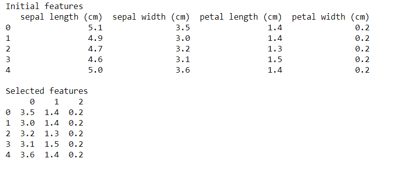
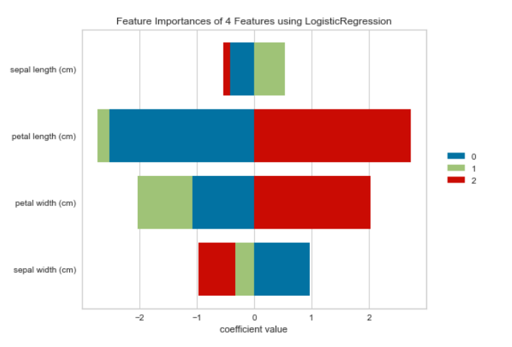
The Recursive feature elimination (RFE) technique has removed the floral leaf length (Sepal Length) from the logistic regression model, as seen within the output. The length of the sepals is that the least essential characteristic/feature.

5. Forward Feature Elimination:

Forward feature Elimination is the opposite of Backward Feature elimination where we look for and find the best features that will help in improving the performance of the model.

Steps:

• We start with one feature. In essence, we train the model n times with each feature individually.
• The variable that gives the best performance is selected as the initial variable
• Then we continue the cycle, each time adding a new variable. The variable that results in the greatest improvement in performance is kept.
• The approach will be continued until the model's performance has significantly improved.

Implementation:

import pandas as pd
from sklearn.datasets import load_iris
from sklearn.feature_selection import f_classif
from sklearn.feature_selection import SelectKBest

iris = load_iris()
data = iris.data
target = iris.target

X_selected = SelectKBest(f_classif, k=3).fit_transform(data, target)

print('F-values: ', f_classif(data,target)[0])
print()
print('Initial features')
print(pd.DataFrame(data, columns=iris.feature_names).head())
print()
print('Selected features')
print(pd.DataFrame(X_selected).head())

Lets check the output of the following code:

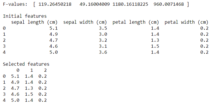
The forward feature selection procedure picked the sepal length, petal length, and petal width that had higher F-values, as shown in the output.

With this article at OpenGenus, you must have the complete idea of Types of Dimensionality Reduction Techniques.