Bayesian Belief Networks

Open-Source Internship opportunity by OpenGenus for programmers. Apply now.

Bayesian Belief Networks also commonly known as Bayesian networks, Bayes networks, Decision Networks or Probabilistic Directed Acyclic Graphical Models are a useful tool to visualize the probabilistic model for a domain, review all of the relationships between the random variables, and reason about causal probabilities for scenarios given available evidence.

This article covers the following topics:

Prerequisite probability concepts for Bayesian Belief Networks:
- Random Variables
- Intersection
- Joint Distribution
- Conditional Distribution
- Conditional Independence
Bayesian Belief Networks and their Components:
- Directed Acyclic Graph
- Conditional Probability Table
Bayesian Belief Networks in Python

1. Prerequisite probability concepts for Bayesian Belief Networks:

As Bayesian Belief Networks are a part of Bayesian Statistics, it is very essential to review probability concepts to fully understand Bayesian Belief Networks. Some essential probability concepts are mentioned below:

Random Variables:

A Random Variable is a set of possible values from a random experiment.
A Random Variable's set of values is the Sample Space.

For Example:

Tossing a coin: we could get Heads or Tails. Let Heads=0 and Tails=1 and Random Variable X represents this event.
X = {0, 1}

giphy-1

The probability of an event happening is denoted by P(x).
The Probability Mass Function(PMF) is f(x) which is the P(X=x).
Therefore f(0) = f(1) = 1/2
Probability of event X not happening is denoted by P(~X) and is equal to 1 - P(X).

Intersection

The probability that Events A and B both occur is the probability of the intersection of X and Y. The probability of the intersection of Events X and Y is denoted by P(X ∩ Y).

Joint Distribution:

A joint probability distribution shows a probability distribution for two (or more) random variables.

For Example:

Let's have 2 coin tosses represented by random variables X and Y.
The joint probability distribution f(x, y) of X and Y defines probabilities for each pair of outcomes. X = {0, 1} and Y = {0, 1}
All possible outcomes are: (X=0,Y=0), (X=0,Y=1), (X=1,Y=0), (X=1,Y=1).Each of these outcomes has a probability of 1/4.
f(0, 0) = f(0, 1) = f(1, 0) = f(1, 1) = 1/4.
This concept can be extended to more than 2 variables as well.

Conditional Distribution:

Sometimes, we know an event has happened already and we want to model what will happen next.

The conditional probability of two events X and Y as follows:
P(Y|X) = P(X ∩ Y)/P(X)

For Example:

Yahoo’s share price is low and Microsoft will buy it.
It is cloudy and it might rain.

Conditional Independence

The concept of Conditional Independence is Backbone of Bayesian Networks. Two events are said to be conditionally independent if the occurrence of one event doesn't affect the occurrence of the other event.

For example let one event be the tossing of a coin and the second event be whether it is raining outside or not.

The above mentioned events are conditionally independent as if it rains or not doesn't affect the probability of getting heads or tails.

To read more about Bayesian Statistics and the Bayesian Model, I would highly recommend that you read:

Basic Data Science concepts everyone needs to know by OpenGenus Foundation
Bayesian model by Prashant Anand

2. Bayesian Belief Networks and their Components:

Bayesian Belief Networks are simple, graphical notation for conditional independence assertions.
Bayesian network models capture both conditionally dependent and conditionally independent relationships between random variables.
They also compactly specify the joint distributions.
They provide a graphical model of causal relationship on which learning can be performed.

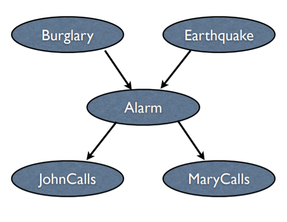
Let us consider the below mentioned example to explain Directed Acyclic Graphs and Conditional Probability Tables:

Let us consider a problem where:

There is an Alarm in a house, which can be set of by 2 events: Burglary and Earthquake with certain conditional probabilities.
The owner of the house has gone for work to office.
The 2 neighbors are Mary and John, who call the owner if they hear an alarm go off with certain conditional probabilities.

Directed Acyclic Graph:

Each node in a Directed Acyclic Graph (DAG) represents a random variable. These variables may be discrete or continuous valued. These variables may correspond to the actual attribute given in the data.

Alarm

Directed: The connections/edges denote cause->effect relationships between pairs of nodes. For example Burglary->Alarm in the above network indicates that the occurrence of a burglary directly affects the probability of the Alarm going off (and not the other way round). Here, Burglary is the parent, while Alarm is the child node.
Acyclic: There cannot be a cycle in a Bayesian Belief Network. In simple English, a variable A cannot depend on its own value – directly, or indirectly. If this was allowed, it would lead to a sort of infinite recursion which we are not prepared to deal with.
Disconnected Nodes are Conditionally Independent:
Based on the directed connections in a Bayesian Belief Network, if there is no way to go from a variable X to Y (or vice versa), then X and Y are conditionally independent. In the example pairs of variables that are conditionally independent are {Mary Calls, John Calls} and {Burglary, Earthquake}.
It is important to remember that ‘conditionally independent’ does not mean ‘totally independent’. Consider {Mary Calls, John Calls}. Given the value of Alarm (that is, whether the Alarm went off or not), Mary and John each have their own independent probabilities of calling. However, if you did not know about any of the other nodes, but just that John did call, then your expectation of Mary calling would correspondingly increase.

Conditional Probability Table:

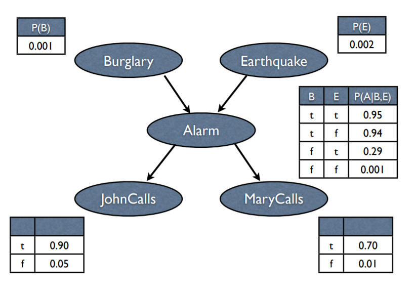
In statistics, the conditional probability table (CPT) is defined for a set of discrete and mutually dependent random variables to display conditional probabilities of a single variable with respect to the others (i.e., the probability of each possible value of one variable if we know the values taken on by the other variables).

-The CPTs for the aforementioned example are:

Alarm-CPT

The CPTs are given already and don't need to be calculated.

Calculation of the occurrence of an Event:

Occurrence of an event can be calculated using the CPTs, DAG and concepts of probability.

As we Disconnected Nodes are Conditionally Independent. Let us now try to calculate the probability that the Alarm rings (A) given that:

John Calls (J)
Mary Calls (M)
Earthquake doesn't happen (~E)
Burglary doesn't happen (~B)

P(A) = P(J|A)*P(M|A)*P(A|~E, ~B)*P(~B)*P(~E) = 0.90*0.70*0.001*0.999*0.998 = 0.00062

3. Bayesian Belief Networks in Python:

Bayesian Belief Networks in Python can be defined using pgmpy and pyMC3 libraries.
Below mentioned are the steps to creating a BBN and doing inference on the network using pgmpy library by Ankur Ankan and Abinash Panda. The same example used for explaining the theoretical concepts is considered for the practical example as well.

Installing pgmpy:

#For installing through anaconda use:
$ conda install -c ankurankan pgmpy

#For installing through pip:
$ pip install -r requirements.txt  # only if you want to run unittests
$ pip install pgmpy

Importing pgmpy:

from pgmpy.models import BayesianModel
from pgmpy.inference import VariableElimination

Defining network structure

alarm_model = BayesianModel([('Burglary', 'Alarm'), 
                              ('Earthquake', 'Alarm'),
                              ('Alarm', 'JohnCalls'),
                              ('Alarm', 'MaryCalls')])

#Defining the parameters using CPT
from pgmpy.factors.discrete import TabularCPD

cpd_burglary = TabularCPD(variable='Burglary', variable_card=2,
                      values=[[.999], [0.001]])
cpd_earthquake = TabularCPD(variable='Earthquake', variable_card=2,
                       values=[[0.998], [0.002]])
cpd_alarm = TabularCPD(variable='Alarm', variable_card=2,
                        values=[[0.999, 0.71, 0.06, 0.05],
                                [0.001, 0.29, 0.94, 0.95]],
                        evidence=['Burglary', 'Earthquake'],
                        evidence_card=[2, 2])
cpd_johncalls = TabularCPD(variable='JohnCalls', variable_card=2,
                      values=[[0.95, 0.1], [0.05, 0.9]],
                      evidence=['Alarm'], evidence_card=[2])
cpd_marycalls = TabularCPD(variable='MaryCalls', variable_card=2,
                      values=[[0.1, 0.7], [0.9, 0.3]],
                      evidence=['Alarm'], evidence_card=[2])

# Associating the parameters with the model structure
alarm_model.add_cpds(cpd_burglary, cpd_earthquake, cpd_alarm, cpd_johncalls, cpd_marycalls)

Checking if the cpds are valid for the model:

alarm_model.check_model()

Output:
True

Viewing nodes of the model:

alarm_model.nodes()

Output:
NodeView(('Burglary', 'Alarm', 'Earthquake', 'JohnCalls', 'MaryCalls'))

Viewing edges of the model:

alarm_model.edges()

Output:
OutEdgeView([('Burglary', 'Alarm'), ('Alarm', 'JohnCalls'), ('Alarm', 'MaryCalls'), ('Earthquake', 'Alarm')])

Checking independency of a node::

alarm_model.local_independencies('Burglary')

Output:
(Burglary | Earthquake)

The entire code can be found on my Github.

Hope you found this article interesting and understood the prerequisite probability concepts, what Bayesian Belief Networks are, and how to represent them in Python.

Bayesian Belief Networks

Machine Learning (ML)

This article covers the following topics:

1. Prerequisite probability concepts for Bayesian Belief Networks:

Random Variables:

Intersection

Joint Distribution:

Conditional Distribution:

Conditional Independence

2. Bayesian Belief Networks and their Components:

Directed Acyclic Graph:

Conditional Probability Table:

Calculation of the occurrence of an Event:

3. Bayesian Belief Networks in Python:

Further Readings:

Binary Space Partitioning Trees

Complex number in C Programming language