
Get this book -> Problems on Array: For Interviews and Competitive Programming
This article will discuss about the Depthwise Convolution operation and how it is implemented using the TensorFlow framework (tf.nn.depthwise_conv2d).
Depthwise Convolution is one part of the Depthwise Separable Convolution that comes under the separable convolution techniques. In many neural network architectures depth-wise separable convolutions are preferred over normal convolutions. These kind of convolutions are used in convolutional neural networks (CNNs) designed for mobile and embedded applications. Some of these CNNs are MobileNet, Xception (both of which are owned by Google).
Table of contents:
- Normal Convolution
- Depth-wise Convolution Operation
- Advantages of using Depth-wise Convolutions
- Implementing depth-wise convolution operation (tf.nn.depthwise_conv2d) in Tensorflow
- Differences between tf.nn.depthwise_conv2d and tf.nn.conv2d
Normal Convolution:
Before we deep dive into Depthwise Convolutions, let us have a look at the process of Normal Convolution from a 2D perspective.
An image is not just 2-D, but it also has depth which is the number of channels. An RGB image would have 3 channels. So an RGB image of 15x15 would have the dimensions 15x15x3.
Let us take an image kernel of size 3x3 for performing Convolution. So let us consider one channel and when we perform convolution on it (considering that zero padding and stride of 1 is applied), we obtain an output image of the size 13x13. The output size can be calculated using the formula: n-f+1 where n is the size of input image, f is the filter/kernel size. All the 9 pixels of the kernel undergo scalar multiplication with the pixels of the input image, this continues till the kernel slides over and covers the entire image.
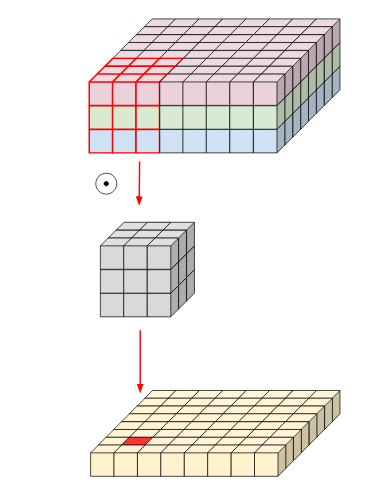
This is for a single channel. But when the input image has 3 channels, the kernel should also have 3 channels, so we'll be doing 3x3x3 i.e 27 multiplications. Finally, what we get is a 13x13x1 image.
We can increase the number of channels by increasing the number of kernels. 'n' kernels would create 'n' images of 13x13x1 dimensions. Then, stack them up to create an image of output 13x13xn. This is accomplished with the help of point-wise convolution by using n 1x1 kernels. But this is an additional step followed after depth-wise convolution in the process of depth-wise seperable convolution, so we will not discuss much about it here.
Depth-wise Convolution Operation:
Now when we come to the depth-wise convolution operation, each channel of the filter is applied at only one channel of the input tensor. This is done by separating the channels of the channels of the input tensor as well as of the kernel and then performing convolution. Finally, all of these are stacked on top back together.
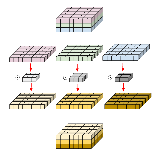
So, when we list out the FLOPs performed for a general case where the input image has the width W, height H and depth C, and a kernel of dimensions KxK is being applied.
As we can see for each channel we will be computing W * H * 1 * K * K FLOPs. Thus, for C number of channels, this becomes W * H * C * K * K FLOPs
Advantages of using Depth-wise Convolutions:
When comparing the performace of a depth-wise convolution to the normal convolution, they're almost similar. But they're efficient when it comes to the number of parameters used and in the number of floating point operations (FLOPs) performed. Like mentioned in the previous section they're followed by a point-wise convolution which in turn significantly reduced the total number of multiplications and thus the operations - this is an advantage in the case where the user wants multiple channels in the output.
However, the number of multiplications done in a normal convolution and a depth-wise convolution remain the same.
Implementing depth-wise convolution operation (tf.nn.depthwise_conv2d) in Tensorflow:
The function parameters of this call are:
tf.nn.depthwise_conv2d(
    input, filter, strides, padding, data_format=None, dilations=None, name=None
)
- input: it is a 4-D tensor with shape according to
data_format. - data_format: The data format for input. Either "NHWC" (default) or "NCHW".
- filter: it is again a 4-D tensor with shape [filter_height, filter_width, in_channels, channel_multiplier].
- strides: it is a 1-D tensor of size 4. Contains the stride of the sliding window for each dimension of input.
- padding: Controls how to pad the image before applying the convolution. Can be the string "SAME" or "VALID" indicating the type of padding algorithm to use, or a list indicating the explicit paddings at the start and end of each dimension. When explicit padding is used and data_format is "NHWC", this should be in the form [[0, 0], [pad_top, pad_bottom],[pad_left, pad_right], [0, 0]]. When explicit padding used and data_format is "NCHW", this should be in the form [[0, 0], [0, 0],[pad_top, pad_bottom], [pad_left, pad_right]].
- dilations: it is a 1-D tensor of size 2. The dilation rate in which we sample input values across the height and width dimensions in atrous convolution. If it is greater than 1, then all values of strides must be 1.
name: A name for this operation (optional).
So, the dimensions of the input, filter and output would be:
- Input:
batch_shape + [height, width, channels]("NHWC") - Filter:
[filter_height, filter_width, in_channels, channel_multiplier] - Output:
[batch, out_height, out_width, in_channels * channel_multiplier]("NHWC")
batch_shape: it is the batch size, it represents the number of images passed together as a group for inference
in_channels: is the total number of channels the filter has.
channel_multiplier: allows us to set the number of different filters we want to apply per channel or dimension. The depth of the output would be multiples of 3.
Please refer to Types of Data Formats in Machine Learning to learn more about the NHWC or NCHW formats.
Usage Example:
>>> import numpy as np
>>> import tensorflow as tf

#Create a 4-D Input Tensor from a 2-D array
>>> x = np.array([[1., 2., 3.],[4., 5., 6.],[7., 8., 9.]], dtype=np.float32).reshape((1, 3, 2, 1))
>>> x
array([[[[1.],
         [2.],
         [3.]],

        [[4.],
         [5.],
         [6.]],

        [[7.],
         [8.],
         [9.]]]], dtype=float32)

#Create a 4D Tensor that represents the kernel/filter
>>> filter = np.array([[1.,2.],[3.,4.]], dtype=np.float32).reshape((2,1,1,2))
>>> filter
array([[[[1., 2.]]],


       [[[3., 4.]]]], dtype=float32)
#Finally apply the depthwise convolution operation
>>> tf.nn.depthwise_conv2d(x, filter, strides=[1, 1, 1, 1], padding='VALID').numpy()
array([[[[13., 18.],
         [17., 24.],
         [21., 30.]],

        [[25., 36.],
         [29., 42.],
         [33., 48.]]]], dtype=float32)
So, finally what we obtain is a 4-D Tensor having the same shape as our input data, here in our case which is "NHWC" format.
Differences between tf.nn.depthwise_conv2d and tf.nn.conv2d
Let us see and understand some of the code samples given in the documentation to compare the differences in their operations
Note that b represents the batch size, (i, j) represents a coordinate in feature map. The only things that are different are the k and q values.
In the depthwise_conv2d operation, the filter dimensions are [filter_height, filter_width, in_channels, channel_multiplier]. The output obtained is,
output[b, i, j, k * channel_multiplier + q] =
    sum_{di, dj} input[b, strides[1] * i + rate[0] * di,
                          strides[2] * j + rate[1] * dj, k] *
                 filter[di, dj, k, q]
Here, k represents an input channel and q(0 <= q < channel_multiplier) represents an output channel. Each input channel k is expanded to k*channel_multiplier with different filters. No cross-channel operations are performed.
In the conv2d operation, the filter used is [filter_height, filter_width, in_channels, out_channels]. The output obtained is,
output[b, i, j, k] =
    sum_{di, dj, q} input[b, strides[1] * i + di,
                             strides[2] * j + dj, q] *
                    filter[di, dj, q, k]
In this context, k represents an output channel and q represents an input channel. It sums up among all input channels, meaning that each output channel k is associated with all q input channels by the filter.
Take an example, considering stride is set to 1 and padding is applied
>>>input_size: (_, 15, 15, 3)
>>>filter of conv2d: (3, 3, 3, 8)
>>>filter of depthwise_conv2d: (3, 3, 3, 3)

output of conv2d: (_, 13, 13, 3)
output of depthwise_conv2d: (_, 13, 13, 3*3)
With this article at OpenGenus, you must have the complete idea of Depthwise Convolution op in TensorFlow (tf.nn.depthwise_conv2d).