In this article, we have explored the approach to visualize Neural Network Models in TensorFlow. We have explored how to use TensorBoard.

Introduction to Model Visualization

Unlike traditional programming, machine learning models can be unpredictable and hence tedious to manage. They can be very bulky programs with 500+ lines of code when you are building models from scratch, or they can be 10-20 lines of code if you employ tensorflow, pandas, scikit-learn, kera and other libraries, which have details embeded in them that you might have missed causing the problems in the model.

Programmers, and coders alike, benefit from well structured code that clearly shows the flow of the project. Specifically for machine learning engineers, there is hence a need to visualize the overall flow of our model, to know which tensors are affecting and are affected by what and to see how our model makes a prediction, etc. This also helps when debugging, tuning parameters and fixing problematic code/models. For this purpose, model visualizers are needed to promote more efficient model tuning and training inspection. There are a number of visualizers available. Tensorflow came up with tensorboard, a built-in visualizer. It tracks the tensors, the parameters and metrics and how they change throughout the implementation of the model, and helps the programmer inspect the overall structure of the code. There are more visualizers out there, but in this article we will use the netron neural network visualizer.

Building and Visualising a Model

Building the Model with Keras

When TensorBoard is loaded, multiple dashboards are available for inspection. The graphs dashboard is is the tool needed to visulize and examine our training model and verify that it's functionality matches our intended design. There is also an op-level graph that you can use to see how tensorfloa itself is managing the tensors and executing the code. This op-level graph presents a different way to view your model and presents a unique insight and other ideas to modify your code.

In the rest of this article, we will go over creating a sequential model from the Fashion-MNIST dataset, and visualizing graph diagnostic data in TensorBoard's Graphs dashboard. Then we will use tf.function, a tracing API, to generate graph data for the functions we will generate.

Firstly, we need to load tensorboard as well as import the libraries we will need.

***Duly note that, I am running this script on a jupyter notebook. ***

%load_ext tensorboard # Load the TensorBoard notebook extension

from datetime import datetime
from packaging import version

import tensorflow as tf
from tensorflow import keras

print("TensorFlow version: ", tf.__version__) # prints out the version of tensorflow you have
assert version.parse(tf.__version__).release[0] >= 2, \
    "This notebook requires TensorFlow 2.0 or above."
# >> TensorFlow version:  2.5.0 

import tensorboard
print("TensorBoard version: ", tensorboard.__version__) # prints out the version of tensorboard you have
# >> TensorBoard version:  2.7.0

You will notice an assertion error raised if your tensorflow version is out of data(i.e., later than version 2.0.0), hence you will need to update tensorflow.

Now we will define a simple four-layer sequencial classification model with keras. The first layer flattens the imagine by scaling the input data without affecting the batch size. Then we implement a regular densely-connected Neural Network as the next layer. The dense function essentially implements output = activation(dot(input, kernel) + bias). For keras, we need to give it the dimensions of the output sequence, and the activation function(in our case we will use relu for the second layer in the sequence and later softmax in the fourth layer). The third layer is a Dropout layer that randomly sets some input units to 0 to prevent overfitting. The inputs unchanged are scaled up such that the sum over all inputs is unchanged. The frequency of this manipulation of inputs is set as the rate, to achieve the unchanged cumulative sum of the inputs, the unchanged inputs are scaled up by 1/(1 - rate). The fourth layer us another dense layer with a softmax activation function.

model = keras.models.Sequential([
    keras.layers.Flatten(input_shape=(28, 28)),
    keras.layers.Dense(32, activation='relu'),
    keras.layers.Dropout(0.2),
    keras.layers.Dense(10, activation='softmax')
])

# Configure the model for training
model.compile(optimizer='adam',loss='sparse_categorical_crossentropy',
    metrics=['accuracy'])

Be sure to check the tensorflow website for the full documentation of these functions.

Training the Model

Now, we are going to load and prepare our data, and use it to train our model.

# Load Training Data
(train_images, train_labels), _ = keras.datasets.fashion_mnist.load_data()
train_images = train_images / 255.0

# Define the Keras TensorBoard callback.
logdir="logs/fit/" + datetime.now().strftime("%Y%m%d-%H%M%S")
tensorboard_callback = keras.callbacks.TensorBoard(log_dir=logdir)

# Train the model.
model.fit(train_images, train_labels, batch_size=64, epochs=5, 
    callbacks=[tensorboard_callback])

This will take a little while depending on your data, and or the number of epochs set. Feel free to go make yourself a coffee or stretch!

Visualizing the Model with TensorBoard

If you havent already, quickly install tensorbaord with a the command 'pip install tensorboard', or else we will get an error when we try to launch tensorboard. In your notebook, we will now launch tensorboard using the command Python %tensorboard --logdir logs. At the top, navigate to the Graphs dashboard. This where the overall graph of the model will be.

See below, the graph of our model.

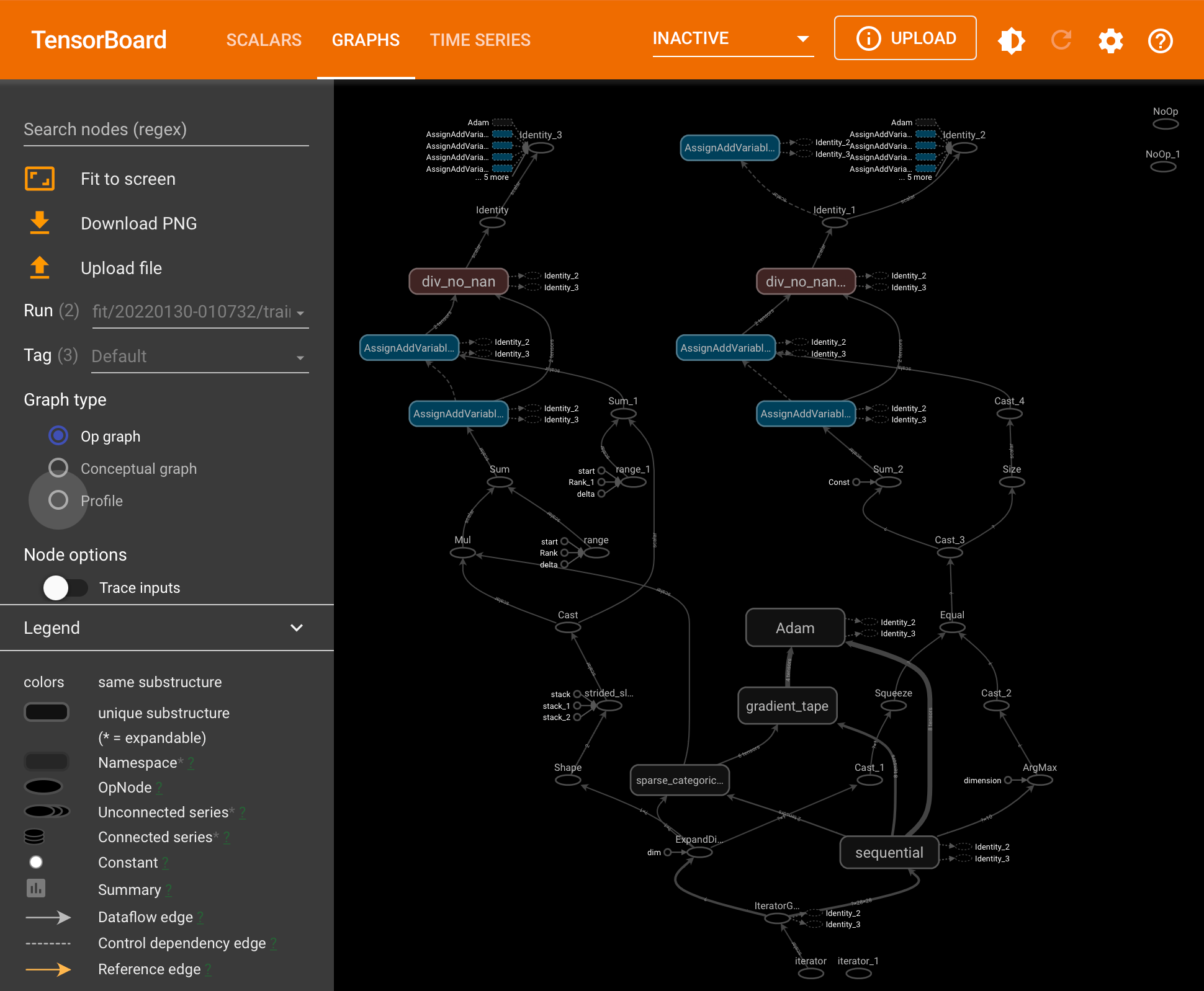
You can see that this clearly maps out our keras model but note that, the flow of data is from bottom to top. You can scroll to zoom, drag to pan and to open nodes you can double click them as shown below.

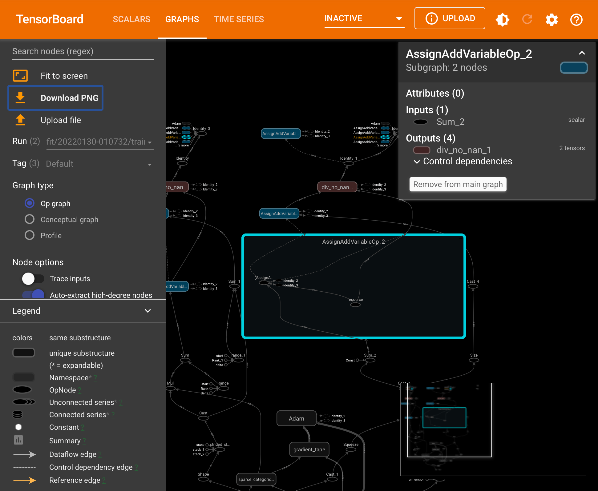
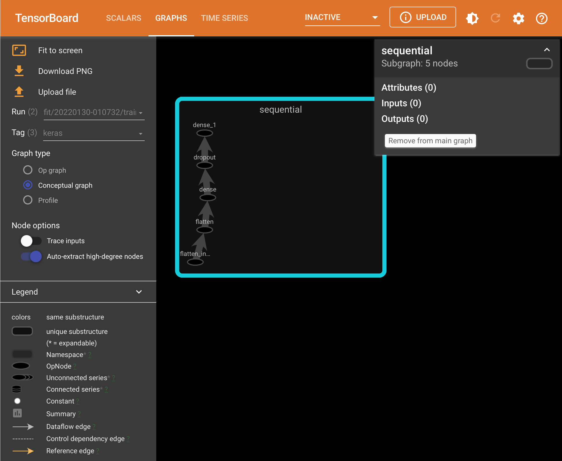
By default, tensorboard opens the Op-Level graph when it loads. As you can see, the Op-Level graph shows the execution of the code, but sometimes we want to see the model itself. That can be seen through the conceptual graph. To see the conceptual graph, on the left of the screen select keras on the list of tag options. You should now be able to toggle conceptual under graph type and see "sequencial". Remember our keras model was a 4 node sequencial model. Double clickling this should confirm the nature of the design of our model. Remember to read from botton to top.

Conclusion

In this article at OpenGenus, we have highlighted the need to visualize our models to produce more efficient code, to understand and visualize the execution of our models and to be able to tune and inspect tensors and other parameters during the course of the execution of out training model.

As a bonus, maybe without realizing, we have also explored the implementation of a keras sequencial model for classification. We defined the dense node, the flatten node and the drop out node.

We then used tensorboard to visualize our code and zoom into suspecious nodes for inspection. In the case where we want to isolate our model itself, we know how to toggle to the conceptual graph and do so.

I encourage exploring other visualizers like netron at netron.app, to see which one seems more comfortable for you and your team.