In this article, we have explored the idea of Graphs in TensorFlow in depth along with details of how to convert function (tf.function) to graph (tf.Graph).

Table of contents:

1. Introduction to Graphs in TensorFlow
2. Creating 'Function' objects with tf.function
3. Converting 'Functions' to Graphs using tf.Graph
4. Conclusion

Introduction to Graphs in TensorFlow

I have spoken at length about the need for visualization of our model and explored one of the ways we can do that. However, there are times when we need to track functions and their computations on each node, on each layer. Tensorflow's tf.Graph is the way to represent the computations of functions. It is a graph that represents the flow of data.

Normally, model are designed such that python executes the code operation by operation and returns the results back to you. This refered to as running the code eagerly. Graph execution is such that the operations are executed as a TensorFlow graph. Intuitively, eager execution is how all programmers code and although eager execution has its advantages, graph execution has its own set of unique advantages as it enables transfer and portability outside the language you're using (in our case python), and tends to have better performance than eager execution.

TensorFlow saves models as graphs when it exports it from python. Therefore this presents the flexibility of using TensorFlow graphs in different environments with/without a python interpretor, like backend servers, mobile phones/tablets and other embeded devices.

Another advantage is the ease of optimizations which allow compilers to do "constant folding". Constant folding is the computation of constant expressions during compilation rather than during execution. For example consider the code below;

x1, y1 = 3.0, 4.0
x2, y2 = 8.4, 5.5

distance = ((y2-y1)**2 + (x2-x1)**2)**0.5
print("Distance = %.3f" % distance)

# >> distance = 5.604

Constant folding allows the compiler to recognize x1,y1 and x2, y2 and store them during compile time as well as the initial distance calculation.

Other tranformations graphs allow the the compile to do are to separate independent sub-computations of a core computation and split them between threads or devices, as well as simplify arithmetic operations by eliminating common subexpressions. TensorFlow has Grappler, which is an entire optimazation systems to perfom these and other optimizations for faster and more efficient models that run fast, run in parallel, and run efficiently on multiple devices.

The graphs generated by the operation are data structures that contain a set of objects. There is the tf.Operations object that represent the list of units for the computations, and the tf.Tensor object that contains the units of data that flow between the computations. Think of graphs as flowcharts of the code execution.

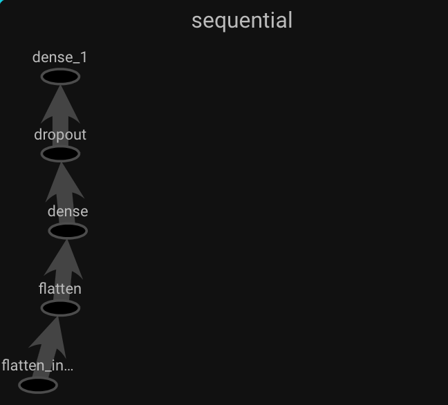
See below an example of a graph which shows the flow(from bottom to top of a 4 layer sequential keras model).

Creating 'Function' objects with tf.function

TensorFlow graphs can be created and run using the tf.function call as a direct call, which takes a function as an input and returns a "Function" object as an output, or as a decorator. A "Function" object builds TensorFlow graphs from the defined function when called and is used the same way as its Python equivalent.

Below we are going to define a regualr function in python and use the tf.function call to allow TensorFlow to take that as an input and return a Function object. We will pass some parameters through both the original python function and the TensorFlow "Function" to see if there's a difference.

# Define a Python function.
def python_function(x, y, c):
  x = tf.matmul(x, y)
  x = x + c
  
  return x

# Converting put function to a TensorFlow "Function"
tensorflow_function = tf.function(python_function)

# Execution
x = tf.constant([[1.0, 2.0]])
y = tf.constant([[2.0], [3.0]])
c = tf.constant(4.0)

result_1 = python_ function(x, y, c).numpy()
result_2 = tensorflow_function(x, y, c).numpy()
print(result_1)
print(result_2)

assert(result_1 == result_2)

# >> [[12.]]
# >> [[12.]]

We see from the output that the results are the same. However, the python_function cannot be represented as a graph unlike the tensorflow_function. See the code below for how to do the same thing but by calling tf.function as a decorator.

# Use the decorator to make `python_function` a `Function`.
@tf.function
def tf_function(x):
  y = tf.constant([[2.0], [3.0]])
  c = tf.constant(4.0)

  return python_function(x, y, c)

x = tf.constant([[1.0, 2.0]])
tf_function(x).numpy()

# >> array([[12.]], dtype=float32)

Converting 'Functions' to Graphs using tf.Graph

One thing we must establish are how TensorFlow graphs interpret python operations. TensorFlow has its own operations, example: tf.matmul(x,y) etc, but python specific operations like if-else clauses, break, continue, return, pass etc cannot be directly changed to a 'Function'. Tensorflow's tf.function has an inbuilt library called AutoGraph (tf.autograph), that converts these operations in python code to graph generating code. See below for an example to illustrate this.

# Define a simple relu function
def relu(x):
  if tf.greater(x, 0):
    return x
  else:
    return 0

# `tf_relu` is a TensorFlow `Function` for `relu`.
tf_relu = tf.function(relu)

print("First branch, with graph:", tf_relu(tf.constant(1)).numpy())
print("Second branch, with graph:", tf_relu(tf.constant(-1)).numpy())

# >> First branch, with graph: 1
# >> Second branch, with graph: 0

# This is the graph-generating output of AutoGraph.
tf.autograph.to_code(relu)

Because of the if-else clause in the relu function, Autograph is needed to generate a graph representation 'Function' from the relu function. The output function is as follows.

print(tf.autograph.to_code(relu))

# Output >>
# def tf__relu(x):
#     with ag__.FunctionScope('relu', 'fscope', ag__.ConversionOptions(recursive=True, user_requested=True, optional_features=(), internal_convert_user_code=True)) as fscope:
#         do_return = False
#         retval_ = ag__.UndefinedReturnValue()

#         def get_state():
#             return (do_return, retval_)

#         def set_state(vars_):
#             nonlocal retval_, do_return
#             (do_return, retval_) = vars_

#         def if_body():
#             nonlocal retval_, do_return
#             try:
#                 do_return = True
#                 retval_ = ag__.ld(x)
#             except:
#                 do_return = False
#                 raise

#         def else_body():
#             nonlocal retval_, do_return
#             try:
#                 do_return = True
#                 retval_ = 0
#             except:
#                 do_return = False
#                 raise
#         ag__.if_stmt(ag__.converted_call(ag__.ld(tf).greater, (ag__.ld(x), 0), None, fscope), if_body, else_body, get_state, set_state, ('do_return', 'retval_'), 2)
#         return fscope.ret(retval_, do_return)

Now to see the graph itself we use the tf.graph callable, see below. I'm not going to paste the entire graph here because it is obnoxiously long, so I suggest you copy and paste the code and run it and see the output graph on your console.

graph = tf_relu.get_concrete_function(tf.constant(1)).graph.as_graph_def()

print("Graph: \n")
print(graph)

# Ouput Graph >>

# Graph: 
# node {
#   name: "x"
#   op: "Placeholder"
#   attr {
#     key: "_user_specified_name"
#     value {
#       s: "x"
#     }
#   }
#   attr {
#     key: "dtype"
#     value {
#       type: DT_INT32
#     }
#   }
#   attr {
#     key: "shape"
# .....

Another element of creating dataflow graphs from tf.functions is Polymorphism, meaning the graph can morph(transform or change the form, structure or, character of) into different graphs. Tensors with a specific dtype and objects with a specific id(), are specialized inputs for tf.Graphs. A new 'Function' with different dtypes and shapes as arguments(input signatures), needs a new tf.Graph. The tf.Graph of the new 'Function' with the new signatures are stored in a ConcreteFunction, which is a wrapper around a tf.Graph.

The code below illustrates this concept. Read the comments as you go along. Copy and paste the code and run it to see the different graphs.

# relu 'Function' created using tf.function decorator
@tf.function
def relu(x):
  return tf.maximum(0., x)

# relu 'Function' creates new graphs as it observes more signatures.
print(relu(tf.constant(5.5)))
print(relu([1, -1]))
print(relu(tf.constant([3., -3.])))


graph1 = relu.get_concrete_function(tf.constant(5.5)).graph.as_graph_def()
graph2 = relu.get_concrete_function([1, -1]).graph.as_graph_def()
graph3 = relu.get_concrete_function(tf.constant([3., -3.])).graph.as_graph_def()

graphs = [graph1, graph2, graph3]

index = 1
for graph in graphs:
    print(f"Graph {index}: \n")
    print(graph)
    index += 1
    
# Ouput >>
# tf.Tensor(5.5, shape=(), dtype=float32)
# tf.Tensor([1. 0.], shape=(2,), dtype=float32)
# tf.Tensor([3. 0.], shape=(2,), dtype=float32)
# Graph 1: ......
# Graph 2: ......
# Graph 3: ......

Note that if the signature doesn't change tf.Graph does not create new graphs. See below for a short example.

print(relu(tf.constant(-2.5))) # Signature matches `tf.constant(5.5)`.
print(relu(tf.constant([-1., 1.]))) # Signature matches `tf.constant([3., -3.])`.

# Since these two signatures have stuctures that are  historically recognized 
# no new graphs are generated

Hence because our relu function can be represented by multiple graphs, it is polymorphic. It supports different input types which require different 'Graphs', and different optimizations for each tf.Graph for better performance. See below for a user friendly output for better understanding.

# Three `ConcreteFunction`s (one for each graph) for 'relu`.
print(my_relu.pretty_printed_concrete_signatures())

# The `ConcreteFunction` also knows the return type and shape!

# Output >>

# relu(x)
#   Args:
#     x: float32 Tensor, shape=()
#   Returns:
#     float32 Tensor, shape=()

# relu(x=[1, -1])
#   Returns:
#     float32 Tensor, shape=(2,)

# relu(x)
#   Args:
#     x: float32 Tensor, shape=(2,)
#   Returns:
#     float32 Tensor, shape=(2,)

Conclusion

Running a code in eager mode has its advantages but when it comes to cross platform and cross environment portablity running in graph mode is the best. In graph mode, functions are converted to 'Function' objects with the tf.function call which are then represented as 'Graph' objects with the tf.Graph call. These graphs are representations of the flow of data and have a 'tf.Operation' object, which represents the units of computations, and a 'tf.tensor' object which represents the units of data that flow between computations.

'Function's can be created via a tf.function() call or by using the @tf.functions decorator. Different input argument attributes require different graphs. Hence a 'Function' that is capable of computing inputs with different attributes(called input signatures) require different 'Graphs'.

When transfered to different environments, tensorflow stores the graphs and transfers them to the other environment where it is then unpacked. Graph mode also allow for better performance in code execution as it uniquely invokes optimization strategies such as constant folding, arithmentic simplification, and computation splitting.