
This article covers Time and Space Complexity of Hash Table (also known as Hash Map) operations for different operations like search, insert and delete for two variants of Hash Table that is Open and Closed Addressing.
Table of contents:
- What is hashing?
- Collision Resolution
2.1. Open Addressing
2.2. Closed Addressing - Time Complexity
3.1. Time Complexity of Searching in Hash Table
3.2. Time Complexity of Insertion and deletion in Hash Table - Space Complexity
As a summary:
Time Complexity For open addressing:
| Activity | Best case complexity | Average case complexity | Worst case complexity |
|---|---|---|---|
| Searching | O(1) | O(1) | O(n) |
| Insertion | O(1) | O(1) | O(n) |
| Deletion | O(1) | O(1) | O(n) |
| Space Complexity | O(n) | O(n) | O(n) |
Time Complexity For closed addressing (chaining):
| Activity | Best case complexity | Average case complexity | Worst case complexity |
|---|---|---|---|
| Searching | O(1) | O(1) | O(n) |
| Insertion | O(1) | O(1) | O(n) |
| Deletion | O(1) | O(1) | O(n) |
| Space Complexity | O(m+n) | O(m+n) | O(m+n) |
where m is the size of the hash table and n is the number of items inserted. This is because linked nodes are allocated memory outside the hash map.
Prerequisites:
What is Hashing?
The process of hashing revolves around making retrieval of information faster. In this, data values are mapped to certain "key" values which aim to uniquely identify them using a hash function. These key-value pairs are stored in a data structure called a hash map. Values can be inserted, deleted, searched and retrieved quickly from a hash map.
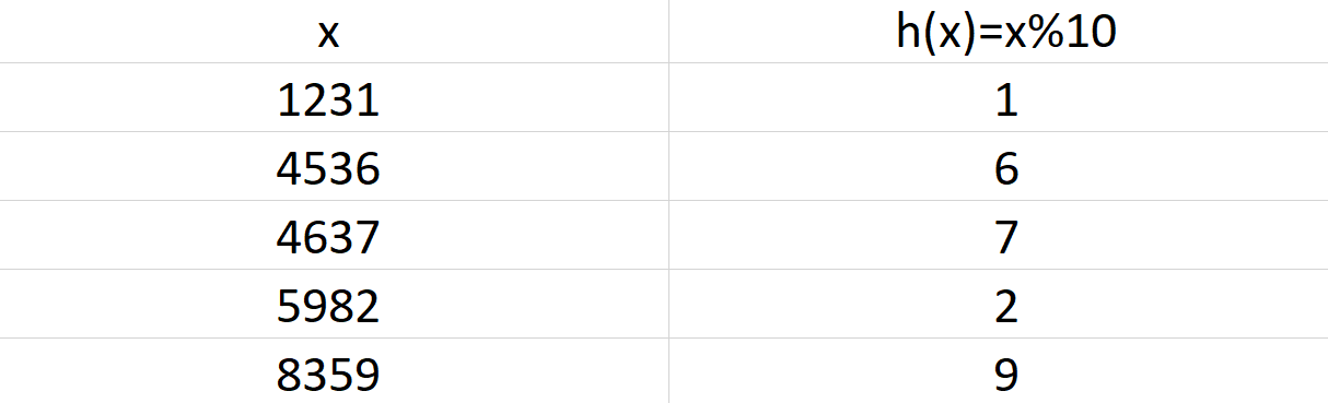
Let's take an example: We are given this array {1231, 4536, 4637, 5982, 8359}. We can select a hash function, which generates keys based on the array values given.
This usually involves a % (mod) operator, among other things.
So, we use a basic hash function defined as: h(x) = x % 10. Here, x represents a value in the array and h(x) is the key obtained.
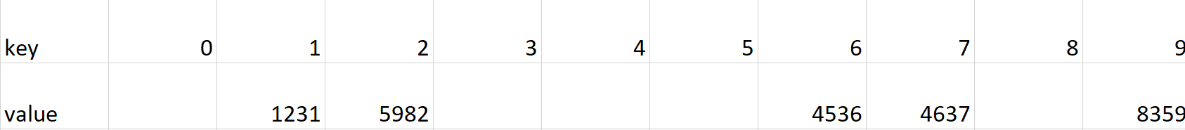
This can be stored in a hash map, where the values are stored in the index denoted by their key values.
C++ STL and Hash Tables
unordered_map < T , T > in C++ is implemented using hash tables in memory.
Collision Resolution
Efficiency of hashing depends on two factors-
- Hashing Function
- Size of the hash table
When hashing functions are poorly chosen, collisions are observed in the table. When multiple values lead to the same key value, then collisions are said to have occurred. Since, we can't overwrite old entries from a hash table, we need to store this new inserted value at a location different than what its key indicates. This adjustment in the hash table to accommodate new values is termed as collision resolution.
There are multiple ways to tackle collisions. The techniques for this are broadly classified under two categories:
- Open Addressing
- Closed Addressing
Open Addressing
The general thought process of this technique is to find a different empty location in the hash table to store the element. This next empty location can be found in a variety of ways such as:
Linear probing
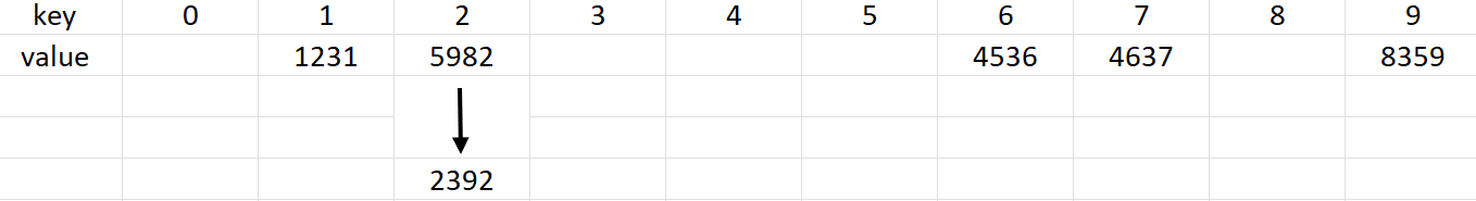
Suppose the hash function is denoted by h(n). Then, for a value k, if the hash generated h(k) is occupied, linear probing suggests to look at the very next location i.e. h(k)+1. When this is occupied as well, we look at h(k)+2, h(k)+3, h(k)+4 and so on... until a vacancy is found. So, we linearly probe through the hash table and insert it at the first available spot. Example: insertion of 2392 in the hash table
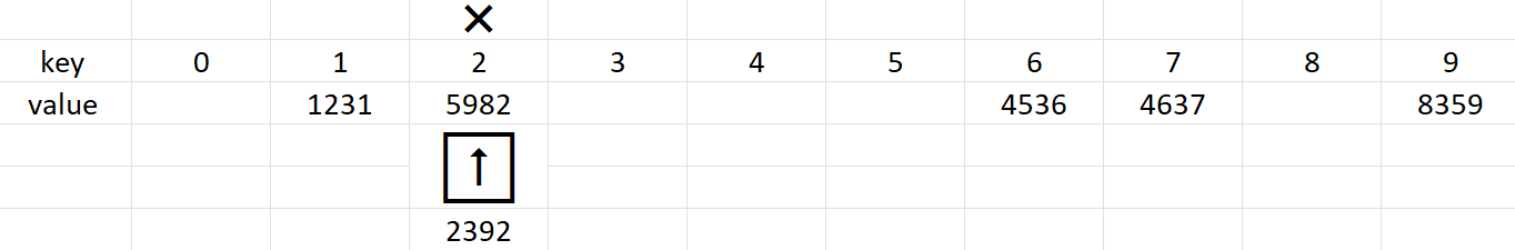
h(2392)=2 but since, this collides with 5982, linear probing dictates checking the location h(k)+1 =2+1 = 3, which is found empty!
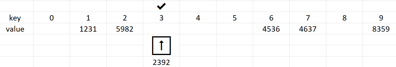
The hash value is usually kept in the range of 1 to size of table using the mod function(%).
During searching, if the element is not found at the key location, the search traverses the hash table linearly stops either if the element is found or if an empty space is found.
However, linear probing leads to clustering of entries in the table, making searches slower and more cumbersome.
Quadratic probing
Very similar to linear probing discussed above, this method of collision resolution searches for the next vacant space by taking steps in the order of i2 where i = 1, 2, 3...
So, the table is traversed in the order h(k)+1, h(k)+4, h(k)+9, h(k)+16 and so on.
Since the step size keeps increasing gradually, the elements are more widely distributed in table, leading to less clustering. But this technique is not entirely free of clustering either.
Double hashing
In this method, we use two hashing functions- h(n) for general hashing and and a new function h'(n) used specifically for resolving conflicts.
So, vacancies are searched in the order as h(k), h(k) + h'(k), h(k) + 2h'(k) and so on...
Advantages and Disadvantages
Open Addressing techniques are highly efficient in memory usage as elements are stored in the space already allocated for the hash table. No extra space is required.
But due to clustering, searching is slower. In the worst case, when the hash table is at full capacity, we would have to check every cell in the hash table to determine if the element exists in the hash table or not.
Closed Addressing
In open addressing techniques, we saw how elements, due to collision, are stored in locations which are not indicated by their keys. So, the next element to be inserted could find its location to be filled, not by an element with which its key collides, but by some other element which was bumped up ahead due to collision. So, in a way, we can picture that a lot of the elements won't be stored at the locations they should have been stored in. This is what makes searching inefficient.
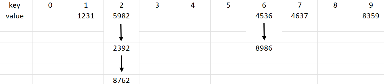
Closed addressing techniques involves the use of chaining of entries in the hash table using linked lists. So, every entry in the hash table leads to a linked list of all the elements that were hashed to a particular key value. The structure is similar to how adjacency lists work in graphs.
So, if in this mode, we wish to insert 2392 in the table, we'd get:
Let's insert 8762 and 8986 in the hash table as well. h(8762)=2 and h(8986)=6 for h(x)=x%10. So, we get:
Advantages and Disadvantages
Advantages of using closed addressing technique is its easy implementation, as well as the surety that if the element is present in the hash table, it will only be found in the linked list at its key. Deletion is also quick and simple in chaining.
But chaining leads to inefficient use of memory as some keys might never be used at all but have still been allocated space in the table. We also need extra memory allocation to store the elements as nodes in the linked list.
In the worst case, chaining can lead to linear time complexity for searching.
Time complexity
Searching
Hashing is a storage technique which mostly concerns itself making searching faster and more efficient.
Best Case
When searching for an element in the hash map, in the best case, the element is directly found at the location indicated by its key. So, we only need to calculate the hash key and then retrieve the element. This is achieved in constant time. So, best case complexity is O(1).
Average Case
If the hashing function is well defined, the probability of values being hashed to the same key falls drastically.
So, in the average case,
- Calculation of hash h(k) takes place in O(1) complexity.
- Finding this location is achieved in O(1) complexity.
- Now, assuming a hash table employs chaining to resolve collisions, then in the average case, all chains will be equally lengthy. If the total number of elements in the hash map is n and the size of the hash map is m, then size of each chain will be n/m. As n/m is a fixed value, we will only have to travel n/m steps at most to find the element. So, in average case, hashing runs in O(1) complexity. This is an definite improvement over binary search O(log n) and linear search O(n).
Worst Case
In the worst case, the hash map is at full capacity. In case of open addressing for collisions, we will have to traverse through the entire hash map and check every element to yield a search result.
In case of chaining, one single linked list will have all the elements in it. So, the search algorithm must traverse the entire linked list and check every node to yield proper search results.
So the worst case complexity shoots up to O(n) since all elements are being checked one by one. Linear searching in worst case is also O(n) whereas binary search still maintains the order of log n in worst case as well.
Insertion and Deletion
Best Case
The hash key is calculated in O(1) time complexity as always, and the required location is accessed in O(1).
Insertion: In the best case, the key indicates a vacant location and the element is directly inserted into the hash table. So, overall complexity is O(1).
Deletion: In the best case, the element to be deleted is found at the key index itself and is directly deleted. This is achieved in constant O(1) complexity.
Average Case
The hash key is calculated in O(1) time complexity and the required location is accessed in O(1).
Insertion: Like we saw in searching earlier, in the average case,all chains are of equal length and so, the last node of the chain is reached in constant time complexity. Here, the new node is created and appended to the list. Overall time complexity is O(1).
Deletion: The node to be deleted can be reached in constant time in the average case, as all the chains are of roughly equal length. Deletion takes place in O(1) complexity.
Worst Case
In the worst cases, both insertion and deletion take O(n) complexity. This is because all nodes are attached to the same linked list due to collision.
Insertion: The entire list of n elements must be traversed to reach the end and then, the new node is appended.
Deletion: The entire list is searched and in the worst case, the element to be deleted is found at the very last node in the last.
Space complexity
In all cases of open addressing, space complexity for hash map remains O(n) where
since every element which is stored in the table must have some memory associated with it, no matter the case.
However,
Summing up:
For open addressing:
| Activity | Best case complexity | Average case complexity | Worst case complexity |
|---|---|---|---|
| Searching | O(1) | O(1) | O(n) |
| Insertion | O(1) | O(1) | O(n) |
| Deletion | O(1) | O(1) | O(n) |
| Space Complexity | O(n) | O(n) | O(n) |
For closed addressing (chaining):
| Activity | Best case complexity | Average case complexity | Worst case complexity |
|---|---|---|---|
| Searching | O(1) | O(1) | O(n) |
| Insertion | O(1) | O(1) | O(n) |
| Deletion | O(1) | O(1) | O(n) |
| Space Complexity | O(m+n) | O(m+n) | O(m+n) |
| where m is the size of the hash table and n is the number of items inserted. This is because linked nodes are allocated memory outside the hash map. |
Thus, in this article at OpenGenus, we have explored the various time complexities for insertion, deletion and searching in hash maps as well as seen how collisions are resolved. Keep learning!