Training, saving and loading Artificial Neural Networks in Keras

Reading time: 30 minutes | Coding time: 15 minutes

In this article, we will explore the concept of saving your own trained neural network models for the future, thereby having to train it only once, and loading it later.

All the code demonstrations are done in Keras, a high level API based on Tensorflow.

Taking an example of Diabetes detection

Let's take an example of a Neural Network built for detecting the presence of diabetes in a patient. The dataset used is the Pima Indian Diabetes dataset.

Importing dependencies

First, let's import the essential libraries

from keras.models import Sequential
from keras.layers import Dense
from keras.models import model_from_json
import numpy as np
import pandas as pd

Fetching and preparing the data

Next, we'll just import the dataset using Pandas and create the input feature vector (X) and target variable (Y)

dataset = pd.read_csv("diabetes.csv")

X = dataset.drop("Outcome",axis=1)
Y = dataset["Outcome"]

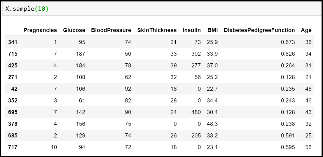
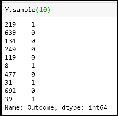
Before we go ahead and train our neural network, let's first have a look at the input features and target variable:

Defining the model structure

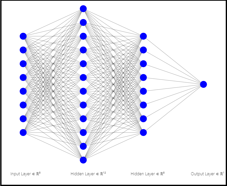
Next, we'll define our simple neural network. The architecture of the neural network has:

• Input layer (8 input features)
• Hidden layer 1 (12 neurons)
• Hidden layer 2 (8 neurons)
• Output layer (1 neuron, softmax function having "0" or "1" as output)

model = Sequential()
model.add(Dense(12, input_dim=8, kernel_initializer='uniform', activation='relu'))
model.add(Dense(8, kernel_initializer='uniform', activation='relu'))
model.add(Dense(1, kernel_initializer='uniform', activation='sigmoid'))

Building the model

Next, we'll build the model using Adam optimizer:

model.compile(loss='binary_crossentropy', optimizer='adam', metrics=['accuracy'])

Training the model

Next, we train the model for 10 epochs

model.fit(X, Y, epochs=10, batch_size=10)

Epoch 1/10
768/768 [==============================] - 0s 134us/step - loss: 0.4180 - acc: 0.8047
Epoch 2/10
768/768 [==============================] - 0s 117us/step - loss: 0.4208 - acc: 0.7943
Epoch 3/10
768/768 [==============================] - 0s 123us/step - loss: 0.4152 - acc: 0.7982
Epoch 4/10
768/768 [==============================] - 0s 122us/step - loss: 0.4077 - acc: 0.8073
Epoch 5/10
768/768 [==============================] - 0s 114us/step - loss: 0.4030 - acc: 0.8138
Epoch 6/10
768/768 [==============================] - 0s 126us/step - loss: 0.4084 - acc: 0.8047
Epoch 7/10
768/768 [==============================] - 0s 118us/step - loss: 0.4079 - acc: 0.8008
Epoch 8/10
768/768 [==============================] - 0s 129us/step - loss: 0.4083 - acc: 0.7995
Epoch 9/10
768/768 [==============================] - 0s 130us/step - loss: 0.4059 - acc: 0.8008
Epoch 10/10
768/768 [==============================] - 0s 118us/step - loss: 0.4139 - acc: 0.8073

Evaluating the model

Finally, let's evaluate our model:

scores = model.evaluate(X, Y, verbose=0)
print("%s: %.2f%%" % (model.metrics_names[1], scores[1]*100))

acc: 80.86%

Now that we have defined, built, trained and evaluate our model, we may feel the need to save it for later, to avoid going through the entire process again.

Saving the model for later

Saving a model requires 2 steps: Saving the model and saving the weights. The model can be saved to a json file using the to_json() function. The weights are saved to a .h5 file using the save_weights() method. Here's a code snippet showing the steps:

model_json = model.to_json()
with open("model.json", "w") as json_file:
    json_file.write(model_json)

model.save_weights("model.h5")

Once these steps are run, the .json and .h5 files will be created in the local directory. These can be used to load the model as it is in the future. These files are the key for reusing the model.

Loading the model

Now that the model has been saved, let's try to load the model again and check for accuracy. This is shown in the code snippet below:

file = open('model.json', 'r')
loaded  = file.read()
file.close()

loaded_model = model_from_json(loaded)
loaded_model.load_weights("model.h5")

It is important to note that you must always compile a model again after loading it, in order for it to run.

loaded_model.compile(loss='binary_crossentropy', optimizer='adam', metrics=['accuracy'])

Accuracy check on loaded model

Here, we will try and achieve the same accuracy score on our loaded model as we got earlier, i.e. 80.86%.

score = loaded_model.evaluate(X, Y, verbose=0)
print("%s: %.2f%%" % (loaded_model.metrics_names[1], score[1]*100))

acc: 80.86%

Hence, we can verify that the performance of our loaded model is exactly same as the model we spent time training. This shows that for other models as well, we can conveniently save a model after training on a large dataset and come back to it later to resume to the same state as earlier.

What we have done, saving a model for later is not limited to one's own models. Keras supports Transfer learning, allowing us to access pre-trained models by others, thus greatly reducing the amount of time and effort we need to spend.

What is Transfer learning?

Traditionally, in order to train a model with good enough accuracy, we needed to have a large size of the dataset, enough time (a few weeks), and sufficient computational power. This is no longer the case with the approach of Transfer learning. Once a model is trained by someone, the pre-trained model can be used by anyone else for solving their problem using this approach.

Transfer learning basically allows us to use either some or all layers of a neural network originally trained for some other purposes.

Keras allows free and open access to a variety of pre trained models, which anyone can use for training their own modified models with minimal computational effort.

Transfer learning will be the next driver of ML success - Andrew Ng

Question