Value Iteration Algorithm (with a 1D example)

In this article, we have explored Value Iteration Algorithm in depth with a 1D example. This algorithm finds the optimal value function and in turn, finds the optimal policy. We will go through the basics before going into the algorithm.

Every Markov Decision Process (MDP) can be defined as a tuple: <S, A, P, R> where

• S: State
• A: Action
• P: Transition function, which is often represented using a table where P(s’| s, a) is probability of reaching a state s’ given action a from an initial state s
• R: Reward which is represented using R(s, a), where R(s, a) is the cost or reward of taking action a in state s

Here, we would require a sequence of actions. But since there is an uncertainity at each step, a direct plan would not work. Hence we would require a sequence of actions at every possible reachable state. This set of actions is called the policy.

Policy is the complete mapping from states to actions. Here, the policy is decided using the Bellman Update Equation as described below

BELLMAN UPDATE EQUATION

According to the value iteration algorithm , the utility U_t(i) of any state i , at any given time step t is given by,

At time t = 0 , U_t(i) = 0
At other time , U_t(i) = max _a[R(i , a) + γ Σ_j U_t-1(j) P(j|i , a)]

The above equation is called the Bellman Update equation. Here, we repeat this equation till the model converges.
(max change in the utility of all the states is less than 𝛿, the bellman factor)

Once the model converges, we run the value iteration algorithm one last time, to determine the policy at that state. Usually, the action that leads to a higher value is preferred.

In the following example, we aim to dry run the value iteration algorithm to get a better understanding of how exactly the algorithm works.

Steps carried out while doing value iteration algorithm

1. Initialise the utilities of all the reachable states as 0.
2. converged=0
3. while(converged==0):
   2.1. Calculate the utility of every state for the next iteration, using the Bellman Update Equation
   2.2. calculate the maximum difference in utility values between the current iteration and the previous iteration
   2.3. If this difference is less than 𝛿, the bellman factor, we say that the model has converged, i.e. converged=1
4. Once the model has converged, run the algorithm once more, but this time, note down the action that resulted in the maximum utility at each state.
5. The set of such actions for each state gives us the policy of the given model.

A SIMPLE 1 DIMENSIONAL EXAMPLE

Dry-run/apply the value iteration algorithm on the following scenario to obtain the optimal policy and the state reward values corresponding to it:

GIVEN PARAMETERS

STATES S

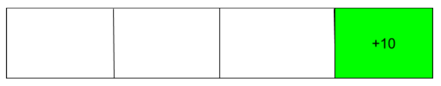
The different states as per the question is as follows:

• S₀
• S₁
• S₂
• S₃

Here , S₃ is an absorbant state with a utility value of 10.

ACTIONS A

The different supported actions are as follows:

• move left (l)

Here the agent moves left with a probability of 0.8 and right with a probability of 0.2

• move right (r)

Here the agent moves left with a probability of 0.2 and right with a probability of 0.8

TRANSITION FUNCTION P

Using the description of the actions, the following transition function can be designed. Here, each box represents P(s'|s,a), i.e. probability of reaching a state s’ given action a from an initial state s

For action l,

T0(s') → FROM(s) ↓	0	1	2	3
0	0.8	0.2	0	0
1	0.8	0	0.2	0
2	0	0.8	0	0.2

For action r,

T0(s') → FROM(s) ↓	0	1	2	3
0	0.2	0.8	0	0
1	0.2	0	0.8	0
2	0	0.2	0	0.8

REWARD FUNCTION

The cost or reward of taking action a in state s, R(s , a) = -1, for all the states and actions. (except state 3, which is the absorbant state)

From	l	r
0	-1	-1
1	-1	-1
2	-1	-1

DISCOUNT FACTOR

The discount factor, γ = 0.25
This efficiently reduces the utility values with each time step, thus ensuring that the model converges faster.

BELLMAN FACTOR

The bellman factor, 𝛿 = 0.01
Once the maximum difference between the state utilities after each time step is less than 𝛿, the model converges.

UTITLITY CALCULATION OF EACH STATE AT EACH TIME PERIOD

Here, the utilities are calculated using the bellman equation as,
U_t(i) = max _a[R(i , a) + γ Σ_j U_t-1(j) P(j|i , a)]

Each table aims to find the net value of each state.
Each element of the table represents U_t-1(j) P(j|i , a) where i is the current state at t-1 and j is the next possible state.
The last row of the table sums up these values and multiplies it with γ.

At time 0, the current state utilities are 0 0 0 10

For state 0,

To	l	r
0	0.8 * 0 = 0	0.2 * 0 = 0
1	0.2 * 0 = 0	0.8 * 0 = 0
2	0 * 0 = 0	0 * 0 = 0
3	0 * 10 = 0	0 * 10 = 0
Net Value	0 * 0.25 = 0	0 * 0.25 = 0

U₁(0) = max( -1+0 , -1+0 ) = -1

For state 1,

To	l	r
0	0.8 * 0 = 0	0.2 * 0 = 0
1	0 * 0 = 0	0 * 0 = 0
2	0.2 * 0 = 0	0.8 * 0 = 0
3	0 * 10 = 0	0 * 10 = 0
Net Value	0 * 0.25 = 0	0 * 0.25 = 0

U₁(1) = max( -1+0 , -1+0 ) = -1

For state 2,

To	l	r
0	0 * 0 = 0	0 * 0 = 0
1	0.8 * 0 = 0	0.2 * 0 = 0
2	0 * 0 = 0	0 * 0 = 0
3	0.2 * 10 = 2	0.8 * 10 = 8
Net Value	2* 0.25 = 0.5	8* 0.25 = 2

U₁(2) = max( -1 + 0.5 , -1 + 2 ) = 1

Maximum Difference: 1.0

At time 1 the current state utilities are -1,-1,1,10

For state 0,

To	l	r
0	0.8 * -1= -0.8	0.2 * -1= -0.2
1	0.2 * -1= -0.2	0.8 * -1= -0.8
2	0 * 1= 0	0 * 1= 0
3	0 * 10 = 0	0 * 10 = 0
Net Value	-1* 0.25 = -0.25	-1* 0.25 = -0.25

U₂(0) = max( -1 + -0.25 , -1 + -0.25 ) = -1.25

For state 1,

To	l	r
0	0.8 * -1= -0.8	0.2 * -1= -0.2
1	0 * -1= 0	0 * -1= 0
2	0.2 * 1= 0.2	0.8 * 1= 0.8
3	0 * 10 = 0	0 * 10 = 0
Net Value	-0.6 * 0.25 = -0.15	0.6 * 0.25 = 0.15

U₂(1) = max( -1 + -0.15, -1 + 0.6 * 0.25 = 0.15 ) = -0.85

For state 2,

To	l	r
0	0 * -1= 0	0 * -1= 0
1	0.8 * -1= -0.8	0.2 * -1= -0.2
2	0 * 1= 0	0 * 1= 0
3	0.2 * 10 = 2	0.8 * 10 = 8
Net Value	1.2 * 0.25 = 0.3	7.8 * 0.25 = 1.95

U₂(2) = max( -1 + 0.3 , -1 + 1.95 ) = 0.95

Maximum Difference: 0.25

At time 2 the current state utilities are -1.25 -0.85 0.95 10

For state 0,

To	l	r
0	0.8 * -1.25 = -1	0.2 * -1.25 = -0.25
1	0.2 * -0.85 = -0.17	0.8 * -0.85 = -0.68
2	0 * 0.95 = 0	0 * 0.95 = 0
3	0 * 10 = 0	0 * 10 = 0
Net Value	-1.17 * 0.25 = -0.292	-0.93 * 0.25 = -0.233

U₃(0) = max( -1 + -0.292 , -1 + -0.233 ) = -1.232

For state 1,

To	l	r
0	0.8 * -1.25 = -1	0.2 * -1.25 = -0.25
1	0 * -0.85 = 0	0 * -0.85 = 0
2	0.2 * 0.95 = 0.19	0.8 * 0.95 = 0.76
3	0 * 10 = 0	0 * 10 = 0
Net Value	-0.81 * 0.25 = -0.203	0.51 * 0.25 = 0.128

U₃(1) = max( -1 + -0.203 , -1 + 0.128 ) = -0.873

For state 2,

To	l	r
0	0 * -1.25 = 0	0 * -1.25 = 0
1	0.8 * -0.85 = -0.68	0.2 * -0.85 = -0.17
2	0 * 0.95 = 0	0 * 0.95 = 0
3	0.2 * 10 = 2	0.8 * 10 = 8
Net Value	1.32 * 0.25 = 0.33	7.83 * 0.25 = 1.958

U₃(2) = max( -1 + 0.33 , -1 + 1.958 ) = 0.958

Maximum Difference: 0.023 < 0.1

At time 3 the current state utilities are -1.232 -0.873 0.958 10

Here, we run the algorithm one last time to determine the policy.

For state 0,

To	l	r
0	0.8 * -1.232 = -0.986	0.2 * -1.232 = -0.246
1	0.2 * -0.873 = -0.175	0.8 * -0.873 = -0.698
2	0 * 0.958 = 0	0 * 0.958 = 0
3	0 * 10 = 0	0 * 10 = 0
Net Value	-1.161 * 0.25 = -0.29	-0.945 * 0.25 = -0.236

U₄(0) = max( -1 + -0.29 , -1 + -0.236 ) = -1.236

For state 1,

To	l	r
0	0.8 * -1.232 = -0.986	0.2 * -1.232 = -0.246
1	0 * -0.873 = 0	0 * -0.873 = 0
2	0.2 * 0.958 = 0.192	0.8 * 0.958 = 0.766
3	0 * 10 = 0	0 * 10 = 0
Net Value	-0.794 * 0.25 = -0.199	0.52 * 0.25 = 0.13

U₄(1) = max( -1 + -0.199 , -1 + 0.13 ) = -0.87

For state 2,

To	l	r
0	0 * -1.232 = 0	0 * -1.232 = 0
1	0.8 * -0.873 = -0.698	0.2 * -0.873 = -0.175
2	0 * 0.958 = 0	0 * 0.958 = 0
3	0.2 * 10 = 2	0.8 * 10 = 8
Net Value	1.302 * 0.25 = 0.326	7.825 * 0.25 = 1.956

U₄(2) = max( -1 + 0.326 , -1 + 1.956 ) = 0.956

Maximum Difference: 0.004

At time 4 the current state utilities are -1.236 -0.87 0.956 10

Here the policy is

STATE	PREFERRED ACTION
S0	move left(l)
S1	move left(l)
S2	move left(l)
S3	NA

FINAL UTILITY VALUES AT EACH TIME PERIOD

t	Ut(S0)	Ut(S1)	Ut(S2)	Ut(S3)	Difference
0	0	0	0	10	0
1	-1	-1	1	10	1
2	-1.25	-0.85	0.95	10	0.25
3	-1.232	-0.873	0.958	10	0.023
4	-1.236	-0.87	0.956	10	0.004
5	-1.236	-0.871	0.956	10	0
6	-1.236	-0.87	0.956	10	0

OBSERVATIONS

Here, we observe that going right is always the best option, at any state. Therefore, the policy is to always move right, irrespective of the initial state.

CODE (in python)

nos = 4  # no of states
A = ['l', 'r']  # actions
noa = 2

# R [from state][action]
R = [[-1, -1], [-1, -1], [-1, -1]]

# P [from state] [to state] [action]
P = [
    [[0.8, 0.2], [0.2, 0.8], [0, 0], [0, 0]],
    [[0.8, 0.2], [0, 0], [0.2, 0.8], [0, 0]],
    [[0, 0], [0.8, 0.2], [0, 0], [0.2, 0.8]],
]

delta = 0.01
gamma = 0.25
max_diff = 0

V = [0, 0, 0, 10]  # utilities of each state

print('Iteration', '0', '1', '2', '3', 'Maximum difference', sep="|")

for time in range(0, 30):
    print(time, V[0], V[1], V[2], V[3], max_diff, sep="|")
    Vnew = [-1e9, -1e9, -1e9,10]
    for i in range(3):
        for a in range(noa):
            cur_val = 0
            for j in range(nos):
                cur_val += P[i][j][a]*V[j]
            cur_val *= gamma
            cur_val += R[i][a]
            Vnew[i] = max(Vnew[i], cur_val)
    max_diff = 0
    for i in range(4):
        max_diff = max(max_diff, abs(V[i]-Vnew[i]))
    V = Vnew
    if(max_diff < delta):
        break

# one final iteration to determine the policy
Vnew = [-1e9, -1e9, -1e9, 10]
policy = ['NA', 'NA', 'NA', 'NA']
for i in range(3):
    for a in range(noa):
        cur_val = 0
        for j in range(nos):
            cur_val += P[i][j][a]*V[j]
        cur_val *= gamma
        cur_val += R[i][a]
        if(Vnew[i] < cur_val):
            policy[i] = A[a]
            Vnew[i] = max(Vnew[i], cur_val)
print("The policy is:", policy)

On running this, we get the final table that has the utilities of each state.

Feel free to change the values of the given parameters to observe the changes in the policy.

In this article at OpenGenus, you should have a complete idea of Value Iteration Algorithm. Enjoy.