An adversarial example is an item or input which is slightly modified but in such a way that it does not look different from the original example but the machine learning model misclassifies it. The modifications to the original examples are done in such a way that the user is unable to tell the difference but the model produces incorrect output.

Understand the basics of Adversarial Examples and why it makes Machine Learning models fail 🤮

In this article, we see why adversarial examples are not bugs but are features of Machine Learning models.

Key points:

• Adversarial examples arise due to the presence of non-robust features.
• The non-robust features are captured within a theoretical framework and their widespread existence is established in standard datasets.
• Phenomena observed in practice is due to a misalignment between the human definition of robustness and the inherent geometry of the data.

Hypothesis:

Adversarial vulnerability is a direct result of our models' sensitivity to well-generalising features in the data

Implications

• Explains adversarial transferability, which means that adversarial perturbations computed for one model can transfer to other independently-trained models
• Attributes adversarial vulnerability to a human-centric phenomenon

Previous hypotheses:

Adversarial examples are aberrations that arise because of

1. The high dimensional nature of the input space
2. Statistical flunctuations in the training datas
   Impact: Adversarial robustness is treated as a goal to be disentangled and pursued independently from maximimising accuracy, by (1) improving standard regularisation methods and (2) pre/post-processing of network inputs/outputs

Definitions:

Adversarial examples: Natural inputs that induce erroneous predictions in classifiers
Features: derived from patterns in the data distribution
Non-robust features: Highly predictive features that are brittle and thus incomprehensible to humans

Why do adversarial perturbations arise?

As classifiers are trained to only maximise distributional accuracy, they use any available signal to do so regardless of whether it is comprehensible to humans, as they are indifferent to any other predictive feature. The "non-robust" features can lead to adversarial perturbations.

Implementation 1: Finding robust and non-robust features

Robust features can be disentangled from non-robust features in standard image classification sets.

• A robustified version for robust classification can be constructed for any training set, where standard training on a training set yields good robust accuracy on the original, unmodified test set, implying that adversarial vulnerability is a property of the dataset.
• A non-robust version for standard classification can be constructed for a training dataset with input similar to the original, but seemingly "incorrectly labeled".Inputs are associated to their labels through small adversarial perturbations and only use non-robust features - perturbations can arise from flipping features in the data useful for classifying correct inputs

Robust features model

Setup:

• Binary classification is used, input-label pairs (x,y) that belong to (X x {+/- 1}) are sampled from a data distribution D.
• The goal is to learn a classifier C: X towards {+/- 1}, which will produce a label y corresponding to a given input.

Constraints

• A feature maps from the input space X to the real numbers

• A set of all features is F = {f : X -> R}, the features in F are scaled for mean = 0, var = 1 for the following definitions to be scale-invariant

• Useful, robust and non-robust features:

  • p-useful: a feature is p-useful (p>0) for a given distribution D if it is correlated with the true label in expectation and p_(D)(f) as the largest p for which feature f is p-useful under distribution D, i.e.
    
  • y-robustly useful features: f is a robust feature if under adversarial perrtubation, f remains y-useful. It is also a robustly useful feature f(p_(D)(f)>0) for y > 0. I.e.
    
  • Useful, non-robust features: fetures that re p-useful for p bounded away from 0, but not a y-robust feature for any y>=0 - they help with classification in standard settings but hinder accuracy in adversarial settings as the correlation with the label can be flipped

• The classifier used in classfication tasks to predict the label y is shown as follows.
  

Training

The classifier was trained by minimising a loss function with empirical risk optimisation - which decreased with the correlation between weighted combination of the features of the label

Standard training

• No distinction exists between robust and non-robust features when minimising classification loss - only the p-usefulness matters
• The classifier will use any p-useful feature in F to decrease the loss of the classifier

Robust training

• In the presence of an adversary, any useful but non-robust features can be made anti-correlated with the true label - leads to adversarial vulnerability, so the effect of the adversary must be explicitly accounted for
• The above implies that ERM is no longer sufficient to train robust classifiers, so an adversarial loss function should be used
• In other words, the classifier can no longer learn a useful but non-robust combination of features

Finding robust and non-robust features model

• This is based on the framework that both robust and non-robust features exist that constitute useful signals for standard classifications
• Two datasets will be constructed as follows

Dataset 1 : Robustified dataset

• Samples that primarily contain robust features
• Robust classifiers can be trained using standard training
• Implication 1: Robustness can arise by removing certain features from the dataset, i.e. the new dataset contains less information about the original training set
• Implication 2: Adversarial vulnerability is caused by non-robust features, not inherently tied to the standard training framework

Dataset 2 : Input-label association based purely on non-robust features

• Dataset appears completely mislabeled to humans
• Can train a classifier with good performancce on the standard test set
• Implication 1: Natural models use non-robust features to make predictions even with the presence of robust features
• Implication 2: Non-robust features alone are sufficient for non-trivial generalisations performance on natural images - non-robust features are valuable features, not artifacts of finite-sample overfitting

Side-by-side experiment setup

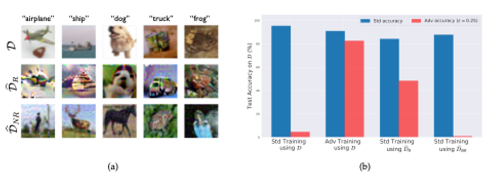
On the left are random examples from the variants of the CIFAR--10 [Kri09] training set: the original training set; the robust training set D_R, restricted to features used by a robust model; and the non-robust training set D_NR, restricted to features relevant to a standard model (labels appear incorrect to humans).

On the right are standard and robust accuracy on the CIFAR-10 test set (D) for models training with: (i) standard training (on D); (ii) standard training on D_NR; (iii) adversarial training (on D); and (iv) standard training on D_R. Models training on D_R and D_NR reflect the original models used to create them: notably, standard training on D_R yields nontrivial robust accuracy.

Disentangling robust and non-robust features

In order to manipulate the features of networks which may be complex and high-dimensional, a robust model can be leveraged and the dataset modified to contain only relevant features

• A robust model C can be used to construct a distribution D_R to satisfy the following conditions:
  

• A training set D_R can be constructed with one to one mapping of x to x_r from the original training set for D. x is the original input and g is the mapping from x to the representation layer. All features in F_C can be enforced to have similar values for x and x_r:
  
  Results: A classifier is trained with standard training then tested on the original data set D. The classifier learned using the new dataset attained good accuracy in standard and adversarial settings.

Non-robust features suffice for standard classification

• Hypothesis: A model trained solely on non-robust features can perform well on the standard test set
• Implementation: Dataset where only features useful for classification are non-robust, formally:
  
• A Dataset D_rand should be constructed as follows
  
• And a Dataset D_det as follows
  

The below table shows the test accuracy of classifiers trained on the D, D_rand and D_det training sets

Non-robust features are useful for classification in the standard setting, as standard training on the above datasets generalise to the original data set

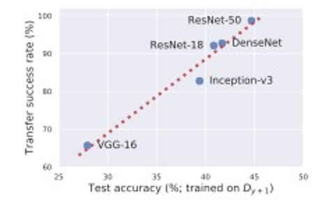
The above figure demonstrates the transfer rate of adversarial examples from a ResNet-50 to different architectures alongside test set performance of these architecture when trainined on the dataset generated in Section 3.2. Architectures more suspectible to transfer attackes also performed better on the standard test set supporting the hypothesis that adversarial transferability arises from utilising similar non-robust features.

Transferability can arise from non-robust features

Adversarial examples transfer across models with different architectures and independently sampled training sets

Setup: Train five different architectures for a standard ResNet-50

Hypothesis: Architectures which learn better from this training set compared to the standard test set are more likely to learn similar non-robust features to the original classifier

Implementation 2: Studying (Non)-Robust Features

A concrete classification task for the purpose of studying adversarial examples and non-robust features, based on Tsipras et al as it contains a dichotomy between robust and non-robust features

Summary:

• Separating Gaussian distributions
• Can precisely quantify adversarial vulnerability as the difference between the intrinsic data geometry and the adversary's perturbation set
• Classifier from using robust training corresponding to a combination of the intrinsic data geometry and the adversary's perturbation set
• Gradients of standard models can be more misaligned with the inter-class direction

Setup:

Problem - maximum likelihood classification between two Gaussian distributions, i.e.
given samples (x, y) from D

the goal is to learn parameters Theta = (mu, Sigma)

with l(x; mu, Sigma) representing the Gaussian negative log-likelihood function

Classification under this model can be accomplished via likelihood test: for unlabeled sample x, we predict y as

Robust analogue of this problem arises from l(x; y.mu, Sigma) with the NLL under adversarial perturbation

Results

1. Vulnerability from metric misalignment - adversarial vulnerability aroses as a misalignment of of two metrics
   
2. Robust Learning
   
   Empical demonstration:
   
   An empirical demonstration of the effect illustrated by Therorem 2 is shown above, as the adversarial pertubation budget e is increased, the learned mean mu remains constant, but the learned covariance blends with the identity matrix, effectively adding more and more uncertainty onto the non-robust feature.
3. Gradient interpretability
   

Implications:

• Adversarial examples are a fundamentally human phenomenon
  • Classifiers exploit highly predictive features that happen to be non-robust under a human-selected notion of similarity (because these features exist in real-world datasets)
  • We cannot expect to have model explanations that are both human-meaningful and faithful to the models themselves as models rely on non-robust features
• For robust, interpretable models, it will be necessary to explicitly encode human priors into the training process

Robustness and accuracy:

• Robustness can be at odds with accuracy - training prevents us from learning the most accurate classifier
• Non-robust features manifest themselves in the same way, yet a classifier with perfect robustness and accuracy is still attainable
• Any standard loss function will learn an accurate yet non-robust classifier
• Classifier learns a perfectly accurate and perfectly robust decision boundary when robust training is employed

Further readings:

• Adversarial Machine Learning by Apoorva Kandpal
• Adversarial examples in the Physical world by Apoorva Kandpal
• Explaining and Harnessing Adversarial examples by Ian Goodfellow by Murugesh Manthiramoorthi
• Deep Neural Networks are Easily Fooled: High Confidence Predictions for Unrecognizable Images by Murugesh Manthiramoorthi