Neural Networks are soft computing systems which aim at simulating the function of the human brain. Since the human brain is fantastic at reasoning, processing and learning in environments of noise, uncertainty and imprecision; implementing Neural Networks allows us to solve very complex, mathematically ill-defined problems using very simple computational operations (such as addition, multiplication, and fundamental logic elements). They are essentially networks consisting of multiple artificial neurons linked together with different connection weights. They are commonly used in pattern recognition, classification, and to find the relationship between the inputs that are fed to a system and its corresponding outputs.

In this article, we will discuss the functioning of a few commonly used Neural Networks, namely:

1. Hebbian Neural Networks
2. Auto-Associative Neural Networks
3. Hopfield Neural Networks
4. Radial Basis Function Neural Networks
5. Kohonen's (Self Organizing Map) Neural Network
6. LVQ (Learning Vector Quantization) Neural Networks

Hebbian Neural Networks

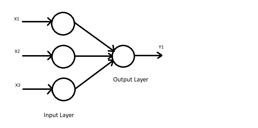
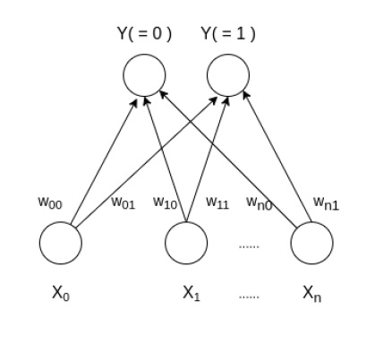
Hebbian Neural Networks, also called Hebb Neural Networks, are one of the simplest types of Artificial Neural Networks. They are feed-forward Neural Networks, meaning that they are unsupervised, since there is no output label associated with the input data during the training process. It consists of one input layer (with multiple input neurons) and one output layer (with a singular output neuron). They work on bipolar data (-1 and 1) and NOT binary data (0 and 1).

These Neural Networks use what is known as Hebb's rule, which states:
If neuron 'A' frequently activates a nearby neuron 'B', then some growth process or metabolic change occurs which makes neuron 'A' more effective at activating neuron 'B'. The inverse also holds true.

Let us now take a look at the training algorithm:
(Assuming that the input vector is Xi, and the target output vector is Y)

1. Initialize all of the weights to 0.
   Thus, Wi = 0
2. Now, update the weights for each training sample.
   Wi(new) = Wi(old) + ∆W,
   where ∆W = Xi + Y (Change in weight depending on how the neurons interact).

Now that the weights have been updated based on the input vector, if we feed the Hebbian Neural Network the same input vector once again, we will find that it outputs '1', meaning that it has successfully recognized the input vector.

Auto-Associative Neural Networks

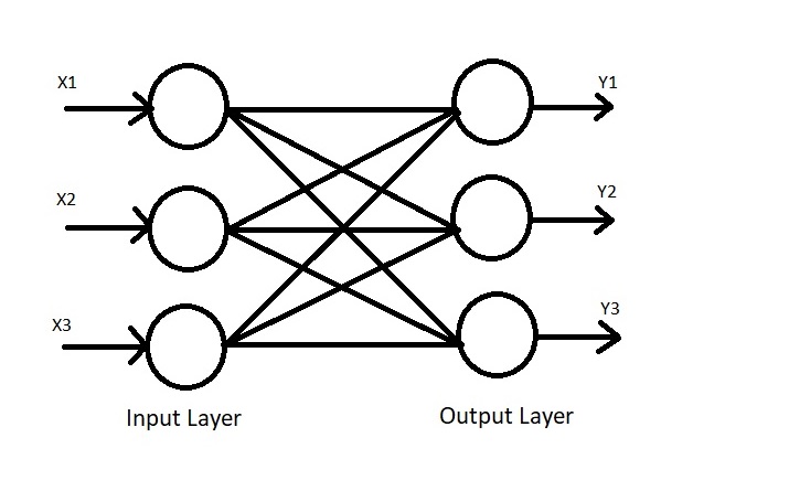
Auto-Associative Neural Networks are used to retrieve a piece of complete data from only a small sample of available data. In order to understand this better, let's turn to a real world example. If a burglar were to commit a crime, and then choose to commit the same crime the next day, only while wearing a face mask this time around (which covers, say, half of the burglar's face), then the concerned authorities will still more than likely be able to deduce that both of these crimes were committed by the same person despite the person's face not being entirely visible on the second day, due to similarities in the way that the crimes were committed and since half of the burglar's face was visible the second time around, the other half can be (approximately) reconstructed. Auto-Associative Neural Networks work in a similar manner. They contain the same number of input as well as output nodes, and also work on bipolar data and not binary data.

Let us now look at a simplified version of the training algorithm:
(Assuming the input vector is Xi, the target output vector is Y, and the weight matrix is Wij)

1. Initialize the weight matrix as:
   Wij = Σ Xi' * Xi, for i=1 to n, and Xi' is Xi transpose.
2. Now, by setting the above weights to the Auto-Associative Neural Network and by
   applying the same input vector,
   Y = Σ Xi * Wij
   We find that the Neural Network obtains an output that is equivalent to the
   input, OR, we can say that the Neural Network has successfully retained
   the pattern.

Now, even if we modify the input vector, that is, if the input vector contains one or two missing or incorrect data entries, we will find that the Neural Network will still be able to recall the complete input pattern.

Hopfield Neural Networks

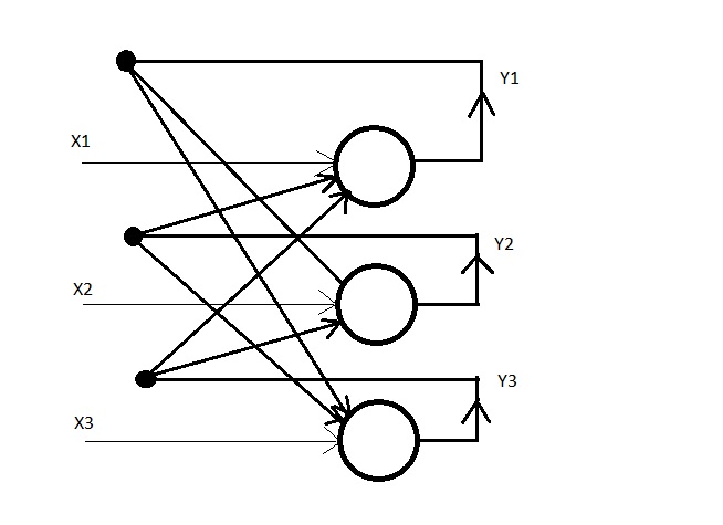
Hopfield Neural Networks are very similar to Auto-Associative Neural Networks. The major difference between the two is that there's an element of back propagation in Hopfield Neural Networks. Here, the output of each neuron (in the output layer) is 'fed back' to every other neuron in the output layer, except itself. Hopfield Neural Networks work with both bipolar as well as binary data.

The training algorithm is essentially the same as that of Auto-Associative Neural Networks, however, there are differences in the testing algorithm, which is as follows:

1. Find the weight matrix with no self connection, i.e. where the diagonal elements
   are 0 owing to the lack of self feedback.
2. Represent the input vector (Xi) in binary.
3. Assign Yi = Xi
4. Find:
   Yin = Xi + Σj[YjWji],
   where Xi represents each individual element in the input vector.

Once we find the value of Yin, it is then broadcasted to every other neuron in the output layer, except itself. If the output vector converges to the required input vector, then we can stop the entire process. If it doesn't converge, we repeat the above processes.

Radial Basis Function Neural Networks

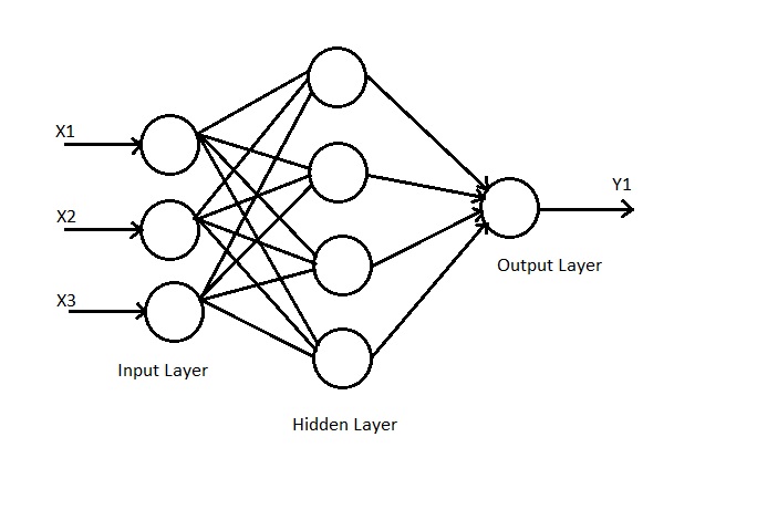
Radial Basis Function (or RBF) Neural Networks, are 3 layer Neural Networks. This means that they have an input layer, a hidden layer, as well as an output layer. These Neural Networks always have MORE neurons in the hidden layer than in the input layer. This allows for an increase in the data's dimensionality, which makes it possible for the Neural Network to separate linearly non-separable data. Thus, Radial Basis Function Neural Networks can, for example, be implemented to find the output of the XOR gate truth table. Each neuron in the hidden layer computes a value via the Gaussian (Radial Basis) Function, as mentioned further below.

Let us take a closer look at the RBF implementation algorithm:

1. Take any input neuron as a receptor neuron.
2. Calculate its Euclidean distance from every other input neuron via:
   r = √[(x2-x1)^2+(y2-y1)^2]
3. Substitute this value of r in the Gaussian function:
   hi(x) = exp(-r^2/2σ^2),
   where σ is the Standard Deviation, which we can assume to be 1 for simplicity.
4. Find:
   ΣWihi(x),
   where Wi represents the weights and hi(x) represents the value that we
   obtained via the above steps.

Once we've applied our activation function to the values of ΣWihi(x), we will find that the Neural Network gives us the necessary output.

Kohonen's Neural Network (Self Organising Map)

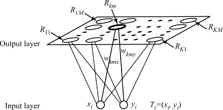
Kohonen's Neural Network, unlike the Radial Basis Function Neural Network, aims at comprehensively visualizing extremely large datasets. This is done so by reducing the dimensionality of the dataset, by grouping the data into multiple clusters. This means that instead of considering the characteristics of each individual data point, we cluster the data together and reference each cluster via a representative data point. All of the elements of that cluster share similar characteristics to that of the representative data point, which means we can deal with a very large number of data points without making a very large number of references. Here, there is an input layer as well as an output layer (Kohonen's layer), but there is NO hidden layer. Every neuron in the input layer is connected to every neuron in the output layer (Kohonen's layer), thus forming a fully inter-connected Neural Network.

The main objective in SOM is to calculate the Euclidean distance of each input data vector to that of the columns of the weight matrix (which represent the clusters), and to find which cluster it is closest to. This means that the input vector belongs to that particular cluster. Thus, we update only that column of the weight matrix (to which the input vector is closest to), as this implies that the centroid of the cluster has moved closer to that particular input vector.

Let us now take a closer look at the steps we need to follow when we implement SOM (Kohonen's NN):

1. Calculate the Euclidean distance of the input vectors from each column of the
   weight matrix (which represents each cluster):
   r = √[(x2-x1)^2+(y2-y1)^2]
2. Pick the winning neuron based on which cluster the input vector is closest
   to, i.e. whichever value of r is smaller.
3. Update that particular weight vector as:
   Wij(new) = Wij(old) + α [Xi - Wij(old)]

These trained weights can then be used to classify new examples.

We now arrive at the final topic of discussion in this article, Learning Vector Quantization (LVQ) Neural Networks!

Learning Vector Quantization (LVQ) Neural Networks

Learning Vector Quantization (LVQ) Neural Networks are very similar to Kohonen's (Self Organizing Map) Neural Networks. The only real difference is in the way that we obtain the weight matrix, and the way in which we update the weights. LVQ is a supervised classification algorithm, since we are aware of the output class label during the training process. In SOM, we start off with a random weight matrix, which we keep updating. In LVQ, however, we form the weight matrix by choosing input vectors that belong to distinct classes.

For example, if our input vectors are:
[1 0 0 1] - Class 1
[1 1 1 1] - Class 2,

then our weight matrix (W) will be:
[1 0
0 1
0 1
1 1]

The rest of the procedure remains largely the same:

1. We find the Euclidean distance of the input vectors from the columns of the weight matrix (which represent the individual clusters), via:
   r = √[(x2-x1)^2+(y2-y1)^2]
2. We then pick the winning neuron based on which cluster the input vector is closest to, i.e. whichever value of r is smaller.
3. Now, we check if the distance that we calculated matches the class label.
4. If it does, then the update rule is as follows:
   Wij(new) = Wij(old) + α [Xi - Wij(old)]
5. If it does not, then the update rule is as follows:
   Wij(new) = Wij(old) - α [Xi - Wij(old)]

These trained weights can then be used to classify new training examples.

Thank you for reading my article on 'Commonly Used Neural Networks' at OpenGenus!