Grouped and Shuffled Grouped Convolution

Abstract

Convolution is an essential mathematical operation being used in many of today's domains including Signal Processing, Image Processing, Probability, Statistics, etc. Naturally, due to its extensive use, improved applications have been developed. So it is imperative that one knows in depth the various ways it can be applied. This article aims at explaining Convolution and the possible ways it can be applied in regards to NNs, CNN to be specific.

Table of contents

1. Introduction to Convolution
2. Grouped Convolution
3. Implementation
4. Shuffled Grouped Convolution
5. Implementation
6. Advantages and Disadvantages
7. Conclusion

Introduction to Convolution

In mathematics, convolution is a mathematical operation on two functions that produces a third function that expresses how the shape of one is modified by the other.

Mathematically this is formulated as,

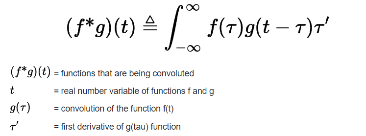
Now we will computationally explore the meaning of this formula one step at a time in matlab.

Consider two randomly generated functions represented by arrays vec1 and vec2.
We can perform convolution on these functions by following,

• Step 1 - Flip the second function (flip_vec2)
• Step 2 - Starting with 1 element aligned from both vec1 and flip_vec2, horizontally shift flip_vec2 until no further elements can be aligned. On each shift sum the element-wise multiplication of the aligned elements.

The resulting vector is the full convolution of vec1 and vec2 which can be computed using,

vec1 = randi([-10, 10], 1, 5)
vec2 = randi([-10, 10], 1, 5)

l1 = length(vec1);
l2 = length(vec2);
full_len = l1 + l2 - 1;
conv_full = zeros(1, full_len);

% step 1
flip_vec2 = fliplr(vec2);

% step 2
for i = 1:full_len
    if i <= l1
        conv_full(i) = sum(vec1(1:i).*flip_vec2(l2 + 1 -i:l2));
    else
        j = l1 + l2 - i;
        conv_full(i) = sum(vec1(l1 + 1 - j:l1).*flip_vec2(1:j));
    end
end

conv_full

If we say the length of the functions vec1 and vec2 is m and n then the length of full convolution will be : m + n - 1

For a test case, the convolution can be graphically visualized as

Another interesting property of full convolution is Commutativeness which is verified by,

l1 = randi([1, 10]);
l2 = randi([1, 10]);
vec1 = randi([-10, 10], 1, l1);
vec2 = randi([-10, 10], 1, l2);

conv_full_12 = conv(vec1, vec2, 'full');
conv_full_21 = conv(vec2, vec1, 'full');

if conv_full_12 == conv_full_21
    disp('Full convolution is commutative')
end

In the application perspective of convolution, it is less informative to find the convolution elements that correspond to less aligned shifts. when we filter the full convolution result and consider only those elements wherein all elements of the smaller function are completely aligned with the larger function we call it valid convolution.

If we say the length of the functions vec1 and vec2 is m and n then the length of valid convolution will be: m - n + 1

Further, as we know the larger function can never be completely aligned with the smaller function, valid convolution IS NOT Commutative

conv_valid_12 = conv(vec1, vec2, 'valid')
conv_valid_21 = conv(vec2, vec1, 'valid')

if conv_full_12 ~= conv_full_21
    disp('Valid convolution is NOT commutative')
end

The corresponding dimensional properties can be extended to higher dimensions.

The same can be done for randomly generated matrices(2d) matlab using,

A_rand = 10*rand(3, 3);
A = round(A_rand, 0);
% creating a symmetric matrix from an unsymmetric one
k_2d = A.*A'

B_rand = 10*rand(8, 8);
M = round(B_rand, 0)

conv_res_valid = conv2(M, k_2d, 'valid')

Here it is important to note that all kernels used for image feature extraction are symmetric. In linear algebra, a symmetric matrix is a square matrix that is equal to its transpose.

The use of symmetric kernels is followed so as to skip the flipping operation, the flipping operation in 2d is nothing but transposing.

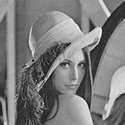
At this point, it is good to play with different kernel settings and observe the results on a sample image file,

I = imread('lenna_grey.png');
imshow(I)
img_dim = size(I)

M_img = im2double(I)

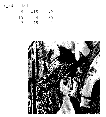
A_rand = randi([-5,5],3, 3);
A = round(A_rand, 0);
k_2d = A.*A'

conv_res_valid_M = conv2(M_img, k_2d, 'valid');
norm_img = normalize(conv_res_valid_M);
imshow(norm_img)

Original image file 'lenna_grey.png'

The resulting kernel's unique feature identification can be seen in a test case,

With a thorough understanding of convolution, we can proceed to brilliant combinatorial applications of Convolution in CNNs.

Grouped Convolution

Grouped Convolution is a technique which combines many convolutions into a single layer, resulting in numerous channel outputs per layer.

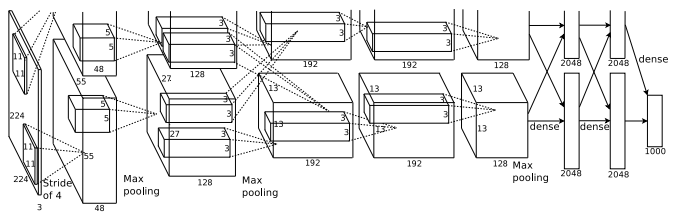
Sometimes also referred to as Filter Groups, the concept of using group convolution was introduced in the AlexNet paper from 2012. This technique was driven by the need to train a network with GPU RAM restrictions. The core concept was to create parallelism in order to reduce single-point load thereby reducing the need for HPC.

In essence, apply different kernels on the same input images and guide it through an equivalent number of pathways (greater than 1) which train and backpropagate in parallel.

To illustrate, consider the below model of 2 pathways used in AlexNet

It is fairly obvious that we do not want to compensate for model performance, likewise, we see that this technique also brings about improvements in accuracy.

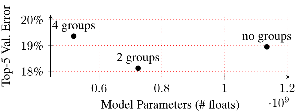
Observing the above image, The error value for a model with 2 groups is notably lower in comparison to a model with none

Looking beyond simple model evaluation metrics, the learning representations of Group convolution are better. The non-subjectiveness is proven by the following findings,

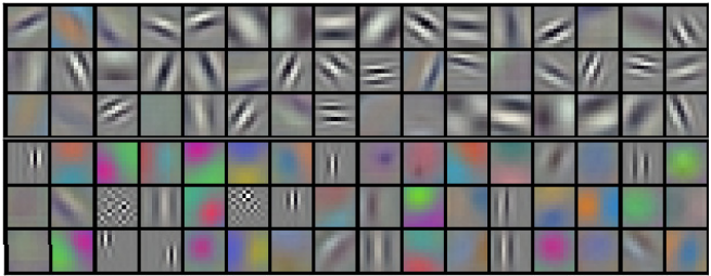
The above image shows the learned information 48 kernels in each of the 2 separate groups, correspondingly trained on different GPUs (say GPU 1 and GPU 2 as in AlexNet). Clear distinctions in both black and white and color information are captured by the different GPUs present.

The use of Group convolution coheres the individual streams into one, this can be comprehended by,

Finally, we can also note that parallelization occurs in two ways:

1. Data parallelism: When the dataset is divided into parts and each chunk is trained on. Each chunk may be thought of as a tiny batch in a mini-batch gradient descent algorithm. More data parallelism can be squeezed out of smaller bits.

2. Model parallelism: Model parallelism is a distributed training strategy that partitions a deep learning model over numerous devices, inside or between instances.

Another interesting feature highlighted in the blog is the convergence of correlations between filters of adjacent layers in a Network-in-Network model trained on CIFAR-10.

Implementation

Logic

First, the fundamental NN architecture parameters must be decided either randomly or based on EDA. When trying to implement grouped convolution, this would also include deciding the number of groups/information channels that the model will learn from. The following actions are then taken to create the group convolution process,

1. Each group is assigned with distinct kernels which it will use to convolve the input.
2. It is made sure that the set of kernels is applied on the same layer so as to learn differently from each level of abstraction.
3. The conventional CNN architecture framework is then created for each group.
   Now this specific layer of the CNN can be put together logically by using the same input and splitting the output into the respective channels.

The code to implement the same will be discussed now,

Code

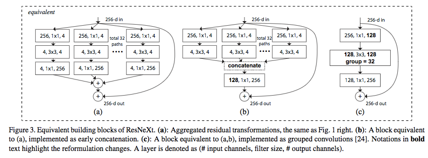
We transition from the use of matlab to python for ease in creating NN models. The below class forms the core part of creating group convolution ResNeXt model,

class ResNeXtBottleneck(nn.Module):

    def __init__(self, in_channels, out_channels, stride, cardinality, base_width, widen_factor):
        """ Constructor
        Args:
            in_channels: input channel dimensionality
            out_channels: output channel dimensionality
            stride: conv stride. Replaces pooling layer.
            cardinality: num of convolution groups.
            base_width: base number of channels in each group.
            widen_factor: factor to reduce the input dimensionality before convolution.
        """
        super(ResNeXtBottleneck, self).__init__()
        width_ratio = out_channels / (widen_factor * 64.)
        D = cardinality * int(base_width * width_ratio)
        self.conv_reduce = nn.Conv2d(in_channels, D, kernel_size=1, stride=1, padding=0, bias=False)
        self.bn_reduce = nn.BatchNorm2d(D)
        self.conv_conv = nn.Conv2d(D, D, kernel_size=3, stride=stride, padding=1, groups=cardinality, bias=False)
        self.bn = nn.BatchNorm2d(D)
        self.conv_expand = nn.Conv2d(D, out_channels, kernel_size=1, stride=1, padding=0, bias=False)
        self.bn_expand = nn.BatchNorm2d(out_channels)

        self.shortcut = nn.Sequential()
        if in_channels != out_channels:
            self.shortcut.add_module('shortcut_conv',
                                     nn.Conv2d(in_channels, out_channels, kernel_size=1, stride=stride, padding=0,
                                               bias=False))
            self.shortcut.add_module('shortcut_bn', nn.BatchNorm2d(out_channels))

    def forward(self, x):
        bottleneck = self.conv_reduce.forward(x)
        bottleneck = F.relu(self.bn_reduce.forward(bottleneck), inplace=True)
        bottleneck = self.conv_conv.forward(bottleneck)
        bottleneck = F.relu(self.bn.forward(bottleneck), inplace=True)
        bottleneck = self.conv_expand.forward(bottleneck)
        bottleneck = self.bn_expand.forward(bottleneck)
        residual = self.shortcut.forward(x)
        return F.relu(residual + bottleneck, inplace=True)

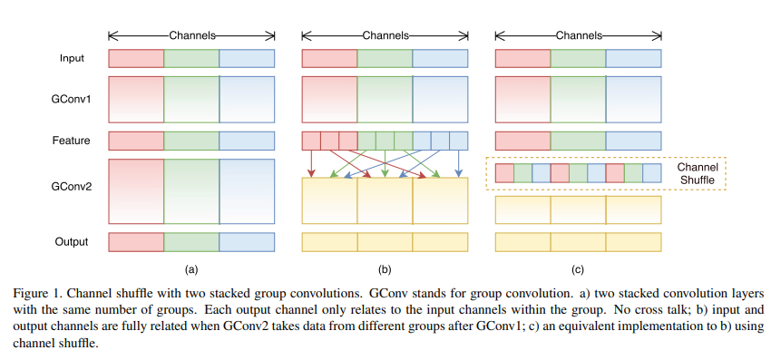
Shuffled Grouped Convolution

In convolutional neural networks, Channel Shuffle is an operation that helps combinatorially decide the information flow between feature channels, and when the infromation is derived from applying group convolution this process is termed as Shuffled Grouped Convolution.

The use of grouped convolution brings about distinct learning segments. Each of these individual segments has kernel-based unique learned information which can be interchangeably combined with successive layers. This concept was first envisioned in ShuffleNet published in 2017.

This concept can be visualized as,

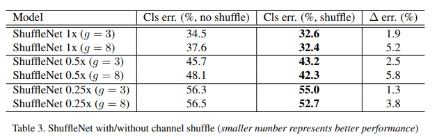
This type of combinatorial model often provides better accuracy which is verified by the following results from ShuffleNet.

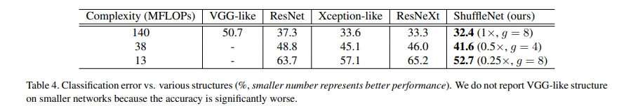
Further, the paper compares the ShuffleNet model with other extremely competitive models, whose results are,

Implementation

Logic

Naturally, it is required to implement grouped convolution before moving on to shuffling the channel information which is done by,

1. Selecting the combination of information segments that are going to be interchanged, usually uniform i.e., each channel of the successive layer obtains one equivalent segment of information from each channel from the previous layer.
2. proceeding this the input for the successive layer is created appropriately following the decided combination.

The code to implement the same will be discussed now,

Code

A baseline Shuffle net block functionality can be achieved in python using,

class ShuffleInitBlock(nn.Module):
    """
    ShuffleNet specific initial block.
    Parameters:
    ----------
    in_channels : int
        Number of input channels.
    out_channels : int
        Number of output channels.
    """
    def __init__(self,
                 in_channels,
                 out_channels):
        super(ShuffleInitBlock, self).__init__()

        self.conv = conv3x3(
            in_channels=in_channels,
            out_channels=out_channels,
            stride=2)
        self.bn = nn.BatchNorm2d(num_features=out_channels)
        self.activ = nn.ReLU(inplace=True)
        self.pool = nn.MaxPool2d(
            kernel_size=3,
            stride=2,
            padding=1)

    def forward(self, x):
        x = self.conv(x)
        x = self.bn(x)
        x = self.activ(x)
        x = self.pool(x)
        return x

class ShuffleNet(nn.Module):
    """
    ShuffleNet model from 'ShuffleNet: An Extremely Efficient Convolutional Neural Network for Mobile Devices,'
    https://arxiv.org/abs/1707.01083.
    Parameters:
    ----------
    channels : list of list of int
        Number of output channels for each unit.
    init_block_channels : int
        Number of output channels for the initial unit.
    groups : int
        Number of groups in convolution layers.
    in_channels : int, default 3
        Number of input channels.
    in_size : tuple of two ints, default (224, 224)
        Spatial size of the expected input image.
    num_classes : int, default 1000
        Number of classification classes.
    """
    def __init__(self,
                 channels,
                 init_block_channels,
                 groups,
                 in_channels=3,
                 in_size=(224, 224),
                 num_classes=1000):
        super(ShuffleNet, self).__init__()
        self.in_size = in_size
        self.num_classes = num_classes

        self.features = nn.Sequential()
        self.features.add_module("init_block", ShuffleInitBlock(
            in_channels=in_channels,
            out_channels=init_block_channels))
        in_channels = init_block_channels
        for i, channels_per_stage in enumerate(channels):
            stage = nn.Sequential()
            for j, out_channels in enumerate(channels_per_stage):
                downsample = (j == 0)
                ignore_group = (i == 0) and (j == 0)
                stage.add_module("unit{}".format(j + 1), ShuffleUnit(
                    in_channels=in_channels,
                    out_channels=out_channels,
                    groups=groups,
                    downsample=downsample,
                    ignore_group=ignore_group))
                in_channels = out_channels
            self.features.add_module("stage{}".format(i + 1), stage)
        self.features.add_module("final_pool", nn.AvgPool2d(
            kernel_size=7,
            stride=1))

        self.output = nn.Linear(
            in_features=in_channels,
            out_features=num_classes)

        self._init_params()

    def _init_params(self):
        for name, module in self.named_modules():
            if isinstance(module, nn.Conv2d):
                init.kaiming_uniform_(module.weight)
                if module.bias is not None:
                    init.constant_(module.bias, 0)

    def forward(self, x):
        x = self.features(x)
        x = x.view(x.size(0), -1)
        x = self.output(x)
        return x


def get_shufflenet(groups,
                   width_scale,
                   model_name=None,
                   pretrained=False,
                   root=os.path.join("~", ".torch", "models"),
                   **kwargs):
    """
    Create ShuffleNet model with specific parameters.
    Parameters:
    ----------
    groups : int
        Number of groups in convolution layers.
    width_scale : float
        Scale factor for width of layers.
    model_name : str or None, default None
        Model name for loading pretrained model.
    pretrained : bool, default False
        Whether to load the pretrained weights for model.
    root : str, default '~/.torch/models'
        Location for keeping the model parameters.
    """

    init_block_channels = 24
    layers = [4, 8, 4]

    if groups == 1:
        channels_per_layers = [144, 288, 576]
    elif groups == 2:
        channels_per_layers = [200, 400, 800]
    elif groups == 3:
        channels_per_layers = [240, 480, 960]
    elif groups == 4:
        channels_per_layers = [272, 544, 1088]
    elif groups == 8:
        channels_per_layers = [384, 768, 1536]
    else:
        raise ValueError("The {} of groups is not supported".format(groups))

    channels = [[ci] * li for (ci, li) in zip(channels_per_layers, layers)]

    if width_scale != 1.0:
        channels = [[int(cij * width_scale) for cij in ci] for ci in channels]
        init_block_channels = int(init_block_channels * width_scale)

    net = ShuffleNet(
        channels=channels,
        init_block_channels=init_block_channels,
        groups=groups,
        **kwargs)

    if pretrained:
        if (model_name is None) or (not model_name):
            raise ValueError("Parameter `model_name` should be properly initialized for loading pretrained model.")
        from .model_store import download_model
        download_model(
            net=net,
            model_name=model_name,
            local_model_store_dir_path=root)

    return net

Advantages and Disadvantages

Advatages

Grouped Convolution

1. NN model width restrictions are removed.
2. Immediate multi-perspective feature extraction allows a higher level of information capture.
3. Parallelism allows for use of far lesser computational resources.
4. Improvements in overall accuracy and segmentwise learning distinction.

Shuffle Group Convolution

Makes use of combinatorial training to improve,

1. Model training
2. Model resource use
3. Model performance

Disadvantages

1. Integrating such aspects requires a good conceptual and computational grasp.
2. Model prerequisites will require careful EDA and intermediatory testing.
3. Because of the complexity, debugging model imperfections will be hard.

Conclusion

With a complete understanding of Convolution, Grouped Convolution, and Shuffle Group Convolution one will be able to greatly appreciate the
nuances and intricacies of modern-day CNN research. The level of abstraction brought by applications of such complex yet logically elegant methods can be broken and the true beauty of basic mathematical operations and their associated influence can be experienced.

Beyond the theoretical decorations, improvements in cognitive ability are brought forward by the effort of trying to successfully implement the discussed concepts.

References

1. A comprehensive understanding of 2d and 3d convolution procedures and visualization can be found in Convolutional Neural Networks (CNN).
2. The full code can for CIFAR-10 and CIFAR-100 can found at ResNeXt
3. A copious number of models can be found from imgclsmob, from where the shuffled group convolution code was derived.