
Get this book -> Problems on Array: For Interviews and Competitive Programming
Reading time: 15 minutes
Machine learning is divided into three categories: supervised learning, unsupervised learning and reinforcement learning.
In supervised learning, we want to find the best model that describes the relationship between two variables – input and output. It is called supervised because we give the learning algorithm correct examples and it will train itself on these data. Giving this data is like a guide for the learning process. For example, image classification problem, in which we want to classify some pictures into some labels. So we give the learning algorithm collections of pictures with correct labels and it will try to find the best model to classify pictures.
But in unsupervised learning, we are concerning about one variable – input. So we will give the learning algorithm a collection of data without any clue about its structure and label. The goal of unsupervised learning is to explore the structure of the data and performs many tasks like compressing, labling and reducing dimenstions of the data.
Clustering
Clustering is the most common unsupervised learning method. It is the process of organizing data into clusters (groups) where the members of some cluster are more similar to each other than to those in other clusters. Clustering has many applications in many fields like data mining, data science, machine learning and data compression. In machine learning, it is usually used for preprocessing data. There are many clustering algorithms: k-means, DBSCAN, Mean-shift and hierarchy clustering.
Hierarchical Clustering
Hierarchical clustering is a method of clustering. In this method, we find a hierarchy of clusters which looks like the hierarchy of folders in your operating system. This hierarchy of clusters will resemble a tree structure and it is called dendrogram (see image below).
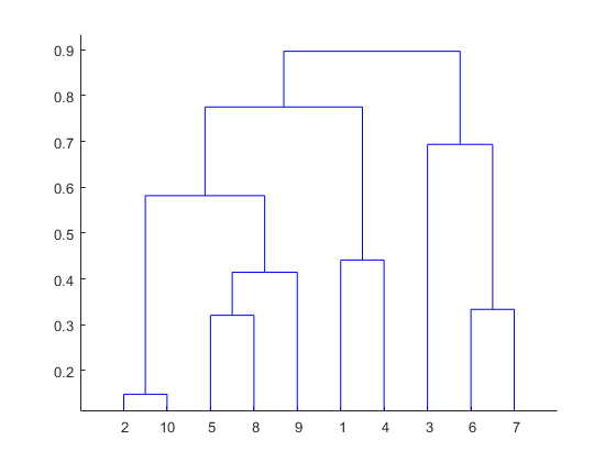
source: https://www.mathworks.com/help/stats/dendrogram.html
Types of Hierarchical Clustering
There are two main methods for performing hierarchical clustering:
-
Agglomerative method: it is a bottom-up approach, in the beginning, we treat every data point as a single cluster. Then, we compute similarity between clusters and merge the two most similar clusters. We repeat the last step until we have a single cluster that contains all data points.
-
Divisive method: it is a top-down approach, where we put all data points in a single cluster. Then, we divide this single cluster into two clusters and recursively do the same thing for the two clusters until there is one cluster for every data point. This method is less common than the agglomerative method.
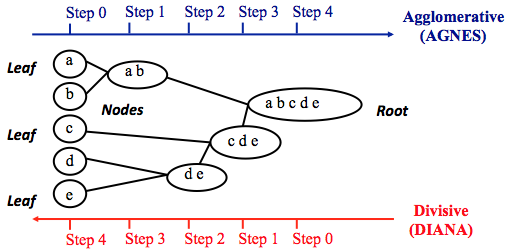
source: https://www.datanovia.com/en/lessons/agglomerative-hierarchical-clustering
Similarity metrics
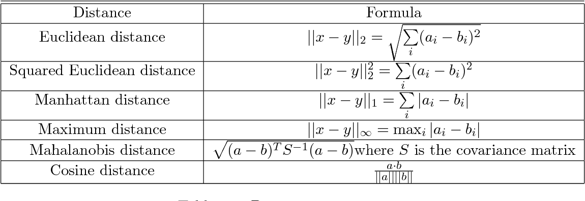
The similarity metric is a function that takes two data points as an input and outputs a value that represents the similarity between them (i.e. the distance between them). The most famous metric is Euclidean distance which is the length of the shortest distance between two data points. Other distance metrics include Manhattan distance, Pearson correlation distance, Eisen cosine correlation distance and Spearman correlation distance. There is no specific right choice for metric, it depends on the problem that we want to solve and the structure of the data.
Linkage methods
There are many ways to determine the distance between two clusters (aka linkage methods):
-
Single linkage: the distance between two clusters is defined as the minimum value of all pairwise distances between the elements of the first cluster and elements of the second cluster.
-
Complete linkage: the distance between two clusters is defined as the maximum value of all pairwise distances between the elements of the first cluster and elements of the second cluster.
-
Average linkage: the distance between two clusters is defined as the average distance between the elements of the first cluster and elements of the second cluster.
-
Centroid linkage: the distance between two clusters is defined as the distance between the centroids of the two clusters.
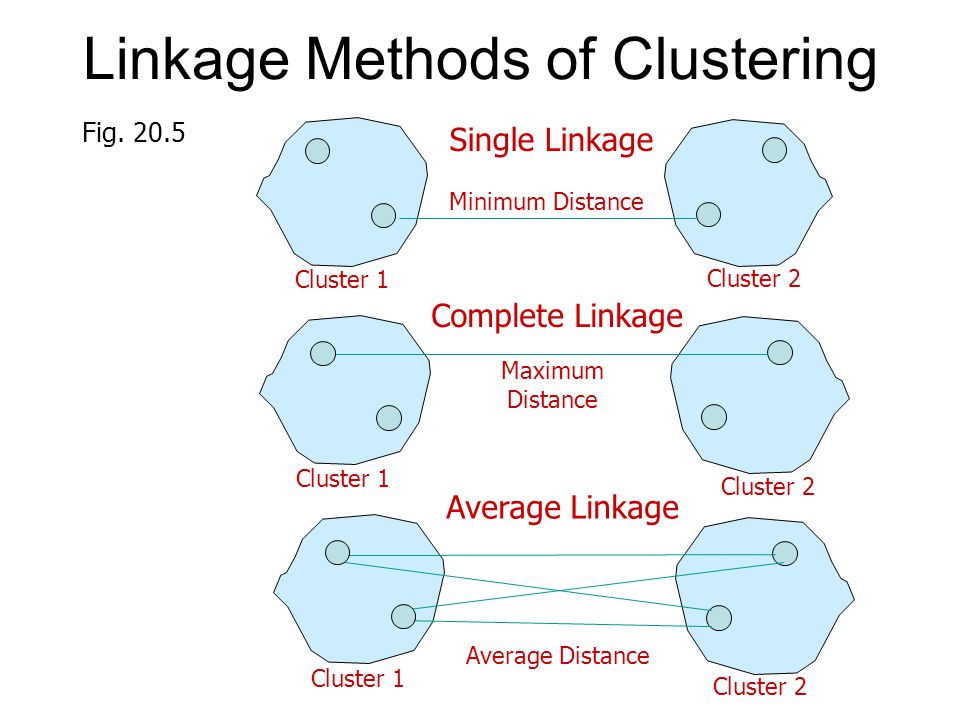
source: https://slideplayer.com/slide/4640145/
Example using python
Prerequisites:
- Python 3.
- Scipy and sklearn
Imports
from sklearn.metrics import normalized_mutual_info_score
from sklearn.datasets.samples_generator import make_blobs
from scipy.cluster.hierarchy import dendrogram, linkage, fcluster
import matplotlib.pyplot as plt
import numpy as np
Generating sample data
make_blobs is used to generate sample data where:
n_samples : the total number of points equally divided among clusters.
centers : the number of centers to generate, or the fixed center locations.
n_features : the number of features for each sample.
random_state: determines random number generation for dataset creation.
This function returns two outputs:
X: the generated samples.
y: The integer labels for cluster membership of each sample.
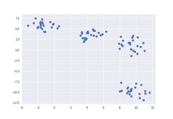
Then we use plt.scatter to plot data points as shown in the figure below.
X, y = make_blobs(n_samples=90, centers=4, n_features=3, random_state=4)
plt.scatter(X[:, 0], X[:, 1])
plt.show()
Clustering
In this part, we are performing agglomerative hierarchical clustering using linkage function from scipy library:
method: is the linkage method, 'single' means the linkage method will be single linkage method.
metric: is our similarity metric, 'euclidean' means the metric will be euclidean distance.
A
(n-1)by 4 matrixZis returned. At the -th iteration, clusters with indicesZ[i, 0]andZ[i, 1]are combined to form cluster with index(n+i). A cluster with an index less thanncorresponds to one of thenoriginal observations. The distance between clustersZ[i, 0]andZ[i, 1]is given byZ[i, 2]. The fourth valueZ[i, 3]represents the number of original observations in the newly formed cluster.
The following linkage methods are used to compute the distanced(s,t)between two clusterssandt. The algorithm begins with a forest of clusters that have yet to be used in the hierarchy being formed. When two clusterssandtfrom this forest are combined into a single clusteru,sandtare removed from the forest, anduis added to the forest. When only one cluster remains in the forest, the algorithm stops, and this cluster becomes the root.
A distance matrix is maintained at each iteration. Thed[i,j]entry corresponds to the distance between clusteriandjin the original forest.
At each iteration, the algorithm must update the distance matrix to reflect the distance of the newly formed cluster u with the remaining clusters in the forest.
for more details check the documentation of linkage function: https://docs.scipy.org/doc/scipy/reference/generated/scipy.cluster.hierarchy.linkage.html
Z = linkage(X, method="single", metric="euclidean")
print(Z.shape)
(89, 4)
Plotting dendrogram
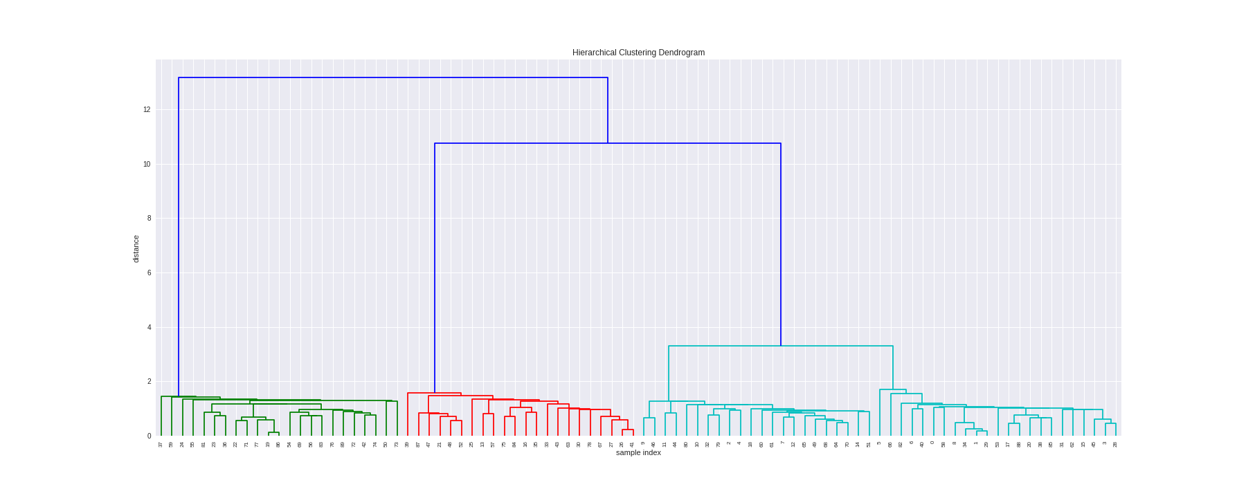
The dedrogram function from scipy is used to plot dendrogram.
- On the x axis we see the indexes of our samples.
- On the y axis we see the distances of our metric ('Euclidean').
plt.figure(figsize=(25, 10))
plt.title("Hierarchical Clustering Dendrogram")
plt.xlabel("Samples indexes")
plt.ylabel("distance")
dendrogram(Z, leaf_rotation=90., leaf_font_size=8. )
plt.show()
Retriving clusters
fcluster is used to retrive clusters with some level of distance.
The number two determines the distance in which we want to cut the dendrogram. The number of crossed line is equal to number of clusters.
cluster = fcluster(Z, 2, criterion="distance")
cluster
array([4, 4, 3, 4, 3, 4, 4, 3, 4, 3, 3, 3, 3, 2, 3, 4, 2, 4, 3, 1, 4, 2, 1, 1, 1, 2, 2, 2, 4, 4, 2, 4, 3, 2, 4, 2, 1, 1, 4, 2, 4, 2, 1, 2, 3, 4, 3, 2, 2, 3, 1, 3, 2, 4, 1, 1, 1, 2, 4, 1, 3, 3, 4, 2, 3, 3, 4, 2, 3, 1, 3, 1, 1, 1, 1, 2, 1, 1, 2, 3, 3, 1, 4, 1, 2, 4, 1, 2, 4, 1], dtype=int32
Plotting clusters
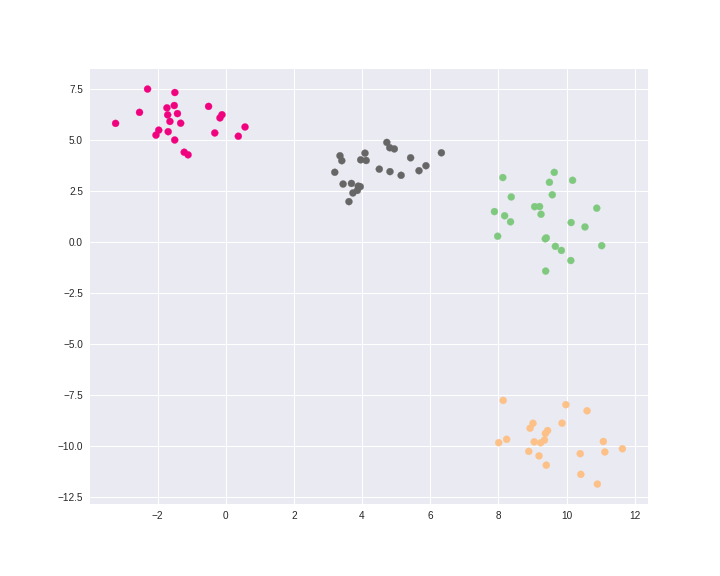
Plotting the final result. Each color represents a different cluster (four clusters in total).
plt.figure(figsize=(10, 8))
plt.scatter(X[:, 0], X[:, 1], c=cluster, cmap="Accent")
plt.show()
Evaluting our clusters
Finally, we will use Normalized Mutual Information (NMI) score to evaluate our clusters. Mutual information is a symmetric measure for the degree of dependency between the clustering and the real classification. When NMI value is close to one, it indicates high similarity between clusters and actual labels. But if it was close to zero, it indicates high dissimilarity between them.
normalized_mutual_info_score(y, cluster)
1.0
The value is one because our sample data is trivial.
Pros and cons
The time complexity of most of the hierarchical clustering algorithms is quadratic i.e. O(n^3). So it will not be efficent for large datasets. But in small datasets, it performs very well. Also it doesn't need the number of clusters to be specified and we can cut the tree at a given height for partitioning the data into multiple groups.