
In today's fast-paced financial landscape, identifying creditworthy borrowers is of paramount importance for lenders and financial institutions. The ability to accurately assess an individual's creditworthiness can significantly impact lending decisions, risk management, and overall financial stability. With the advent of machine learning and data science, credit scoring has witnessed a transformative shift, allowing lenders to leverage advanced algorithms to make more informed and efficient lending choices.
This article developed during my internship at OpenGenus, we will delve into the key components of credit scoring, including the significance of feature selection, data preprocessing, and model evaluation. We will explore the algorithms and models implemented in the repository and understand how they contribute to the overall creditworthiness assessment process. Through this article, I aim to shed light on the diverse array of approaches used to identify creditworthy borrowers, enhance predictive accuracy, and mitigate financial risks.
Table of Content
- Dataset
- Introduction
- Importing the dependencies
- Read the data
- EDA
- Data Preprocessing
- Handling null values
- Imputation with a constant value
- Imputation with mode
- Imputation with k-NN model
- Finding the method with highest accuracy
- Scaling and encoding categorical features
- Clustering
- Handling null values
- Train Test Split
- Model Training
- KNN
- SVM
- MLP
- Logistic Regression
- Decision Tree
- Conclusion based on classification reports
Dataset:
The Statlog German Credit Dataset is a widely used and publicly available dataset that provides valuable insights into credit risk assessment and lending practices. The dataset was created by Prof. Dr. Hans Hofmann in 1994 and is available through the UCI Machine Learning Repository, a renowned repository for machine learning datasets.
The dataset comprises information on credit applications from German banks and consists of 20 attributes, including both numerical and categorical features, making it suitable for various machine learning algorithms. Among the key attributes are the status of existing checking accounts, duration of credit, credit history, purpose of the credit, credit amount, savings account or bonds, present employment status, personal status, and age, among others.
The primary objective of the dataset is to predict whether a credit applicant is "good" or "bad" based on the provided attributes. The "good" or "bad" classification represents the creditworthiness of the applicant, which is crucial for financial institutions to make informed lending decisions and mitigate potential risks.
Click here to access the Statlog German Credit Dataset
Introduction
The objective is to develop a Machine Learning model capable of predicting the credit risk assessment for a given application. This task involves Binary Classification, where the prediction outcome is either "good" or "bad." The dataset comprises a total of 9 variables, consisting of 3 numerical and 6 categorical features, excluding the target column. The significance of this task lies in the necessity to effectively combine these diverse variables and uncover potential underlying relationships. Each subsequent step, from Exploratory Data Analysis to Data Preprocessing and Training the Model, holds equal importance in achieving accurate predictions and meaningful insights.
1. Importing the Dependencies
import pandas as pd
import numpy as np
import seaborn as sns
import matplotlib.pyplot as plt
We will add other dependencies along the way
2. Read the dataset
df = pd.read_csv('/content/german_credit_data (1).csv')
df.head()
Out: 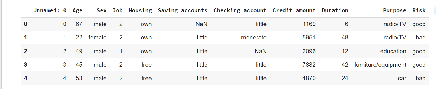
3. EDA
df.info()
Out: 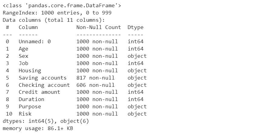
-
Categorical features:
- Sex
- Job
- Housing
- Savings account
- Checking account
- Purpose
- Risk (label)
-
Numerical features:
- Age
- Credit Amount
- Duration
Distribution of sex and risk
fig, axes = plt.subplots(1, 2, figsize=(12, 5))

# Plot for categorical variable 'Sex'
sns.countplot(x='Sex', data=df, ax=axes[0])
axes[0].set_title('Distribution of Sex')

# Plot for categorical variable 'Risk'
sns.countplot(x='Risk', data=df, ax=axes[1])
axes[1].set_title('Distribution of Risk')

plt.show()
Out: 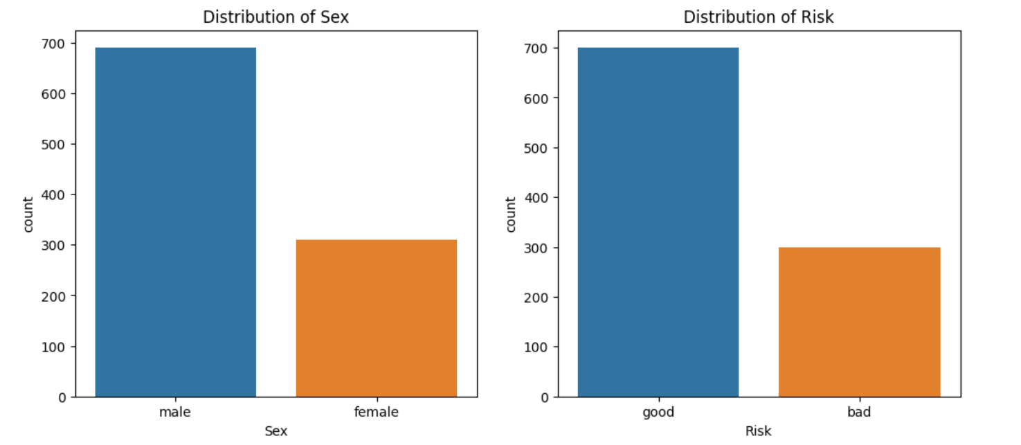
# 'Sex' vs 'Credit amount'
sns.boxplot(x='Sex', y='Credit amount', data=df)
plt.show()
Out: 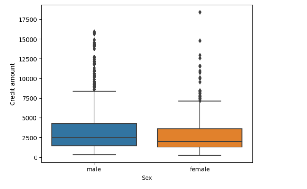
Exploring all categorical features:
# Create a figure and axes with a grid layout
fig, axes = plt.subplots(nrows=2, ncols=3, figsize=(15, 10))

# Categorical Variables
categorical_vars = ['Sex', 'Job', 'Housing', 'Saving accounts', 'Checking account', 'Purpose']

# Plot each categorical variable with respect to 'Risk' in the grid layout
for i, var in enumerate(categorical_vars):
    row = i // 3  # Calculate the row index
    col = i % 3   # Calculate the column index

    sns.countplot(x=var, hue="Risk", data=df, ax=axes[row, col])
    axes[row, col].set_title(f'{var} vs Risk')

# Adjust the spacing between subplots
plt.tight_layout()

# Display the plots
plt.show()
Out: 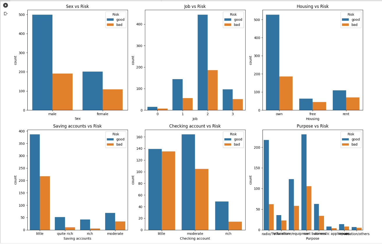
Exploring all numerical features:
# Create a figure and axes with a grid layout
fig, axes = plt.subplots(nrows=1, ncols=3, figsize=(15, 6))

# Numerical Variables
numerical_vars = ['Age', 'Credit amount', 'Duration']

# Plot each numerical variable with respect to 'Risk' in the grid layout
for i, var in enumerate(numerical_vars):
    sns.boxplot(x='Risk', y=var, data=df, ax=axes[i])
    axes[i].set_title(f'{var} vs Risk')

# Adjust the spacing between subplots
plt.tight_layout()

# Display the plots
plt.show()
Out: 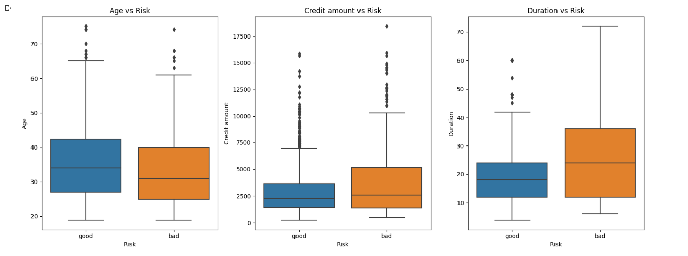
Checking the null values:
df.isnull().sum()
Out: 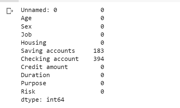
Getting statistical inference of the dataset:
df.describe()
Out: 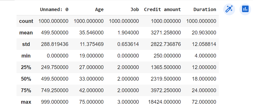
Correlation matrix:
# Heatmap to show correlations
correlation_matrix = df.corr()
sns.heatmap(correlation_matrix, annot=True)
plt.show()
Out: 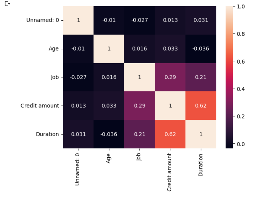
We can observe that only credit amount and duration correlation is greater than 0.5
4. Data Preprocessing
The data preprocessign will include two steps
* handling missing values
* encoding categorical features
4.1 Handling Missing Values
The presence of missing data in the "Saving accounts" and "Checking account" features can significantly impact the performance of a machine learning model. To ensure the accuracy and reliability of the predictive model, it becomes essential to choose an appropriate method for handling these missing values. Three common strategies are considered for this purpose: imputation with a constant value, imputation with mode, and imputation with a k-Nearest Neighbors (k-NN) model.
-
Imputation with a Constant Value:
In this approach, all missing values in the "Saving accounts" and "Checking account" features are replaced with a fixed constant value. The constant value is typically chosen based on domain knowledge or as an indicator of missingness. This method can be straightforward to implement, but it may not capture the underlying relationships in the data, potentially leading to biased predictions. -
Imputation with Mode:
In the mode imputation method, the missing values in each feature are replaced with the most frequent value (mode) observed in that particular feature. By using the mode, the imputed values are aligned with the most common category in the respective feature. This method works well for categorical data like "Saving accounts" and "Checking account" since it preserves the original data distribution and reduces the risk of introducing significant bias. -
Imputation with k-Nearest Neighbors (k-NN) Model:
The k-NN imputation method leverages the k-NN algorithm to estimate missing values based on the values of their k-nearest neighbors in the dataset. This method takes into account the similarity between samples, allowing for more data-driven imputations. By using information from neighboring data points, k-NN imputation tends to capture the local patterns and relationships present in the data, making it potentially more accurate than simple imputation methods.
By comparing the accuracy scores obtained from each method, we can determine which approach yields the best results for our specific dataset and predictive task. The method with the highest accuracy score is likely to be the most suitable choice for handling missing values, as it demonstrates the ability to capture the underlying patterns and contribute to the overall model's predictive power. Through this evaluation process, we can ensure that the chosen imputation method aligns with the dataset's characteristics and enhances the reliability of our machine learning model for credit risk assessment.
4.1.1 Imputation with a constant value
# 1st method -> imputation with a constant value
df_constant = pd.read_csv('/content/german_credit_data (1).csv')

# Filling NaN values with 'Unknown'
df_constant['Saving accounts'].fillna('Unknown', inplace=True)
df_constant['Checking account'].fillna('Unknown', inplace=True)
4.1.2 Imputation with mode
# 2nd method -> imputation with mode
df_mode = pd.read_csv('/content/german_credit_data (1).csv')

# Filling NaN values with mode
df_mode['Saving accounts'].fillna(df_mode['Saving accounts'].mode()[0], inplace=True)
df_mode['Checking account'].fillna(df_mode['Checking account'].mode()[0], inplace=True)
4.1.3 Imputation with k-NN model
# 3rd method -> imputation with k-NN model
from sklearn.preprocessing import OrdinalEncoder
from sklearn.impute import KNNImputer

# Creating an instance of the OrdinalEncoder
encoder = OrdinalEncoder()

# Selecting categorical columns to be encoded
cat_cols = ['Sex', 'Job', 'Housing', 'Saving accounts', 'Checking account', 'Purpose', 'Risk']

# Copying the dataframe to avoid changing the original one
df_encoded = df.copy()

# Encoding the categorical columns
df_encoded[cat_cols] = encoder.fit_transform(df[cat_cols])

# Creating an instance of the KNNImputer
imputer = KNNImputer(n_neighbors=5)

# Applying the imputer
df_encoded = pd.DataFrame(imputer.fit_transform(df_encoded), columns = df.columns)

# Decoding the categorical columns back to their original form
df_encoded[cat_cols] = encoder.inverse_transform(df_encoded[cat_cols])
4.1.4 Finding the method with highest accuracy
# finding which method has highest accuracy

from sklearn.model_selection import train_test_split
from sklearn.linear_model import LogisticRegression
from sklearn.metrics import accuracy_score
from sklearn.impute import SimpleImputer, KNNImputer
from sklearn.preprocessing import OrdinalEncoder

# Assuming df is your DataFrame and 'Risk' is the target variable
df_t = pd.read_csv('/content/german_credit_data (1).csv')
df_t['Risk'] = df_t['Risk'].apply(lambda x: 1 if x=='good' else 0)

# List of imputers
imputers = {
    'constant': SimpleImputer(strategy='constant', fill_value='Unknown'),
    'mode': SimpleImputer(strategy='most_frequent'),
    'knn': KNNImputer(n_neighbors=5)
}

# Initialize encoder
encoder = OrdinalEncoder()

# Splitting the data into train and test sets
X_train, X_test, y_train, y_test = train_test_split(df_t.drop('Risk', axis=1), df_t['Risk'],
                                                    test_size=0.2, random_state=42)

# Iterating over imputers
for name, imputer in imputers.items():
    # Copy the train and test sets
    X_train_imputed = X_train.copy()
    X_test_imputed = X_test.copy()

    # Apply encoding for knn imputer
    if name == 'knn':
        X_train_imputed[['Saving accounts', 'Checking account']] = encoder.fit_transform(X_train_imputed[['Saving accounts', 'Checking account']])
        X_test_imputed[['Saving accounts', 'Checking account']] = encoder.transform(X_test_imputed[['Saving accounts', 'Checking account']])

    # Perform imputation
    X_train_imputed[['Saving accounts', 'Checking account']] = imputer.fit_transform(X_train_imputed[['Saving accounts', 'Checking account']])
    X_test_imputed[['Saving accounts', 'Checking account']] = imputer.transform(X_test_imputed[['Saving accounts', 'Checking account']])

    # If knn, inverse transform after imputation
    if name == 'knn':
        X_train_imputed[['Saving accounts', 'Checking account']] = encoder.inverse_transform(X_train_imputed[['Saving accounts', 'Checking account']])
        X_test_imputed[['Saving accounts', 'Checking account']] = encoder.inverse_transform(X_test_imputed[['Saving accounts', 'Checking account']])

    # One-hot encoding for the categorical features
    X_train_imputed = pd.get_dummies(X_train_imputed)
    X_test_imputed = pd.get_dummies(X_test_imputed)

    # Training the model
    model = LogisticRegression(max_iter=1000)
    model.fit(X_train_imputed, y_train)

    # Predicting the test set results and calculating the accuracy
    y_pred = model.predict(X_test_imputed)
    accuracy = accuracy_score(y_test, y_pred)

    print(f'Imputer: {name}, Accuracy: {accuracy}')
Out: 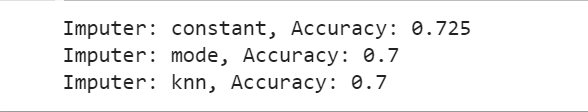
We see that constant imputer has highest accuracy so we'll use that from here on, this is how it looks like,
df_constant.head()
Out: 
4.2 Scaling and encoding categorical features
Scaling all the numerical features to a Log based distribution:
# List of numerical columns to be log transformed
numerical_columns = ['Age', 'Credit amount', 'Duration']

# Apply log(1 + x) transformation to all numerical columns
for col in numerical_columns:
    df_constant[col] = np.log1p(df_constant[col])

# Print the new DataFrame to verify
df_constant.head()
Out: 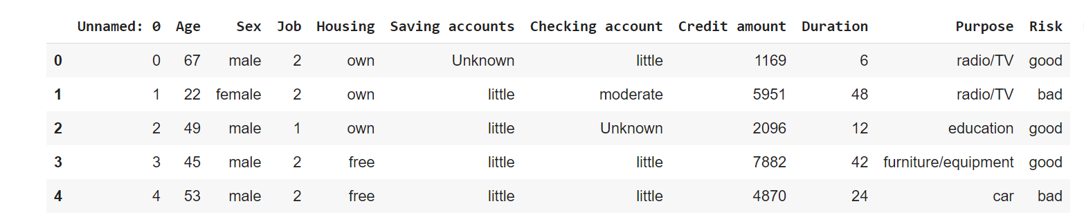
One hot encoding all the categorical features:
# List of categorical columns to be one-hot encoded
categorical_columns = ['Sex', 'Job', 'Housing', 'Saving accounts', 'Checking account', 'Purpose', 'Risk']

# Perform one-hot encoding
df_encoded = pd.get_dummies(df_constant, columns=categorical_columns)

# Print the new DataFrame to verify
df_encoded.head()
Out: 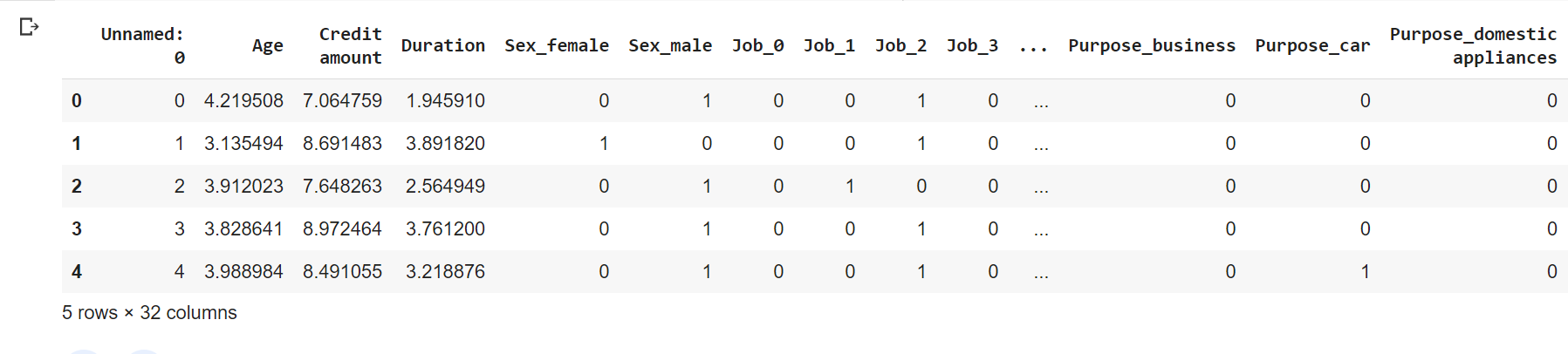
Standardizing numerical columns:
df_excluded = df_encoded.iloc[:, 1:]

from sklearn.preprocessing import StandardScaler

# Create a copy of the DataFrame
df_encoded_copy = df_excluded.copy()

# List of numerical columns
numerical_columns = ['Age', 'Credit amount', 'Duration']

# Create a scaler object
scaler = StandardScaler()

# Apply the scaler only to the numerical columns of the DataFrame copy
df_encoded_copy[numerical_columns] = scaler.fit_transform(df_encoded_copy[numerical_columns])
Now we will perform clustering, clustering is a powerful unsupervised learning technique that aims to group similar data points together based on their inherent characteristics. While clustering is often used as a standalone analysis tool, it can also play a significant role in enhancing the performance of supervised machine learning models. By identifying distinct clusters within the data, we can gain valuable insights into the underlying structure and patterns present in the dataset.
One key advantage of clustering is its ability to create new features that can be used as input for machine learning models. These new features represent the cluster memberships of the data points and can capture additional information about their relationships and proximity to other data points. By incorporating cluster memberships as features, we can potentially improve the model's ability to capture complex interactions and decision boundaries, leading to more accurate predictions.
The Elbow Method for Determining Optimal 'k' in k-means Clustering:
The k-means clustering algorithm is a popular and widely used clustering technique that aims to partition the data into 'k' distinct clusters. However, choosing the optimal value for 'k' is essential, as it directly affects the clustering results. The Elbow Method is a commonly employed technique for determining the optimal value of 'k' in k-means clustering.
The Elbow Method involves running the k-means algorithm for a range of 'k' values and calculating the sum of squared distances (SSD) between data points and their assigned cluster centers. As 'k' increases, the SSD typically decreases, as each data point can be assigned to a more specific and nearby cluster. However, beyond a certain value of 'k', the SSD improvement slows down, and the clusters may start to overfit the data, leading to reduced interpretability and generalization.
The Elbow Method seeks to find the 'k' value at which the SSD improvement begins to flatten out, forming an "elbow" in the plot of SSD versus 'k.' This point represents the optimal trade-off between the number of clusters and the clustering quality.
By employing the Elbow Method, we can determine the most suitable value for 'k' in k-means clustering for our dataset. Once we have identified the optimal 'k,' we can use the resulting clusters as additional features in our supervised machine learning models. This integration of clustering-based features can provide valuable insights into the data structure and enhance the model's ability to capture complex relationships, ultimately leading to improved model performance and more accurate predictions.
from sklearn.cluster import KMeans
import matplotlib.pyplot as plt

# Extract only the numerical columns for k-means clustering
numerical_data = df_encoded_copy[numerical_columns]

# Calculate sum of squared distances
ssd = []
K = range(1,10)  # Check for up to 10 clusters
for k in K:
    km = KMeans(n_clusters=k, n_init = 10)
    km = km.fit(numerical_data)
    ssd.append(km.inertia_)  # Sum of squared distances

# Plot sum of squared distances / Inertia
plt.plot(K, ssd, 'bx-')
plt.xlabel('k')
plt.ylabel('Sum of squared distances')
plt.title('Elbow Method For Optimal k')
plt.show()
Out: 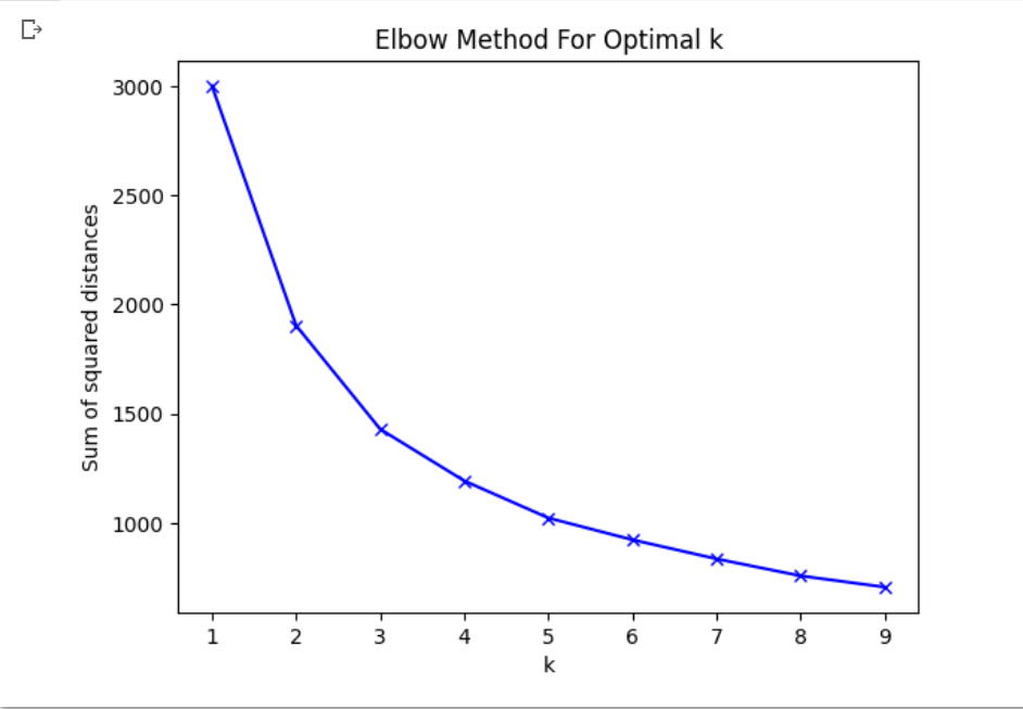
k = 3 seems suitable from the graph so we will use 3 clusters,
from sklearn.cluster import KMeans

# Define the number of clusters
n_clusters = 3

# Create a k-means object and fit it to the numerical data
km = KMeans(n_clusters=n_clusters, random_state=0, n_init = 10)
clusters = km.fit_predict(df_encoded_copy[numerical_columns])
df_encoded_copy['cluster'] = clusters
df['cluster'] = clusters
5. Train Test Split
'train_test_split' function is applied, allocating 20% of the data to the test set and the remaining 80% to the training set. The 'random_state' parameter is set to 42, ensuring the reproducibility of the data split.
from sklearn.model_selection import train_test_split

# Define the features and the target
X = df_final.drop(columns=['Risk_good', 'Risk_bad'], axis=1)
y = df_final['Risk_good']

# Split the dataset into a training and a test set
X_train, X_test, y_train, y_test = train_test_split(X, y, test_size=0.2, random_state=42)
6. Model Training
We will train our dataset on five different models and compare their accuracies to choose the best performing model. The models involved in training are
- KNN
- SVM
- MLP
- Logistic Regression
- Decision Tree
6.1 KNN
K-Nearest Neighbors (KNN) is a simple and intuitive algorithm used in both classification and regression tasks in machine learning. It is a non-parametric and instance-based learning algorithm, which means it doesn't make any underlying assumptions about the data distribution and instead relies on the data points themselves.
In KNN, the "K" refers to the number of nearest neighbors that are considered when making a prediction for a new data point. When a new data point needs to be classified or predicted, the algorithm finds the K closest data points in the training dataset based on some distance metric (commonly Euclidean distance). These K neighbors then vote on the class label in the case of classification or provide their average for regression.
The main idea behind KNN is that data points belonging to the same class or having similar target values are often close to each other in the feature space. Therefore, the class or value of a new data point can be determined based on the majority vote or average of its K nearest neighbors.
Some key characteristics of the KNN algorithm include:
-
Non-linearity: KNN can effectively handle complex and non-linear decision boundaries, making it suitable for datasets with intricate relationships between features and target labels.
-
Lazy learning: KNN is a lazy learning algorithm, meaning that it doesn't build an explicit model during the training phase. Instead, it memorizes the training data to use it during predictions, making the training phase faster and more memory-efficient.
-
Hyperparameter 'K': The choice of the value for 'K' is crucial in KNN. A small 'K' can lead to overfitting, where the model might be too sensitive to outliers and noise, while a large 'K' can result in underfitting, where the model might oversimplify the decision boundaries.
-
Distance Metric: The choice of distance metric can impact the performance of KNN. While the Euclidean distance is commonly used, other distance metrics like Manhattan distance or Minkowski distance can be employed based on the nature of the data and the problem.
It's important to note that KNN's computational complexity can increase significantly with a large number of training samples since it needs to calculate distances for each data point during predictions. Despite this drawback, KNN remains a versatile and straightforward algorithm, particularly suitable for small to medium-sized datasets and as a benchmark model for more complex algorithms.
from sklearn.model_selection import GridSearchCV
from sklearn.neighbors import KNeighborsClassifier
from sklearn.metrics import classification_report, accuracy_score

knn = KNeighborsClassifier()

parameters = {
    'n_neighbors': [3, 5, 7, 9, 11, 13, 15, 17, 19],  # Example values, you can choose others
    'weights': ['uniform', 'distance'],
    'p': [1, 2]  # 1 is manhattan_distance and 2 is euclidean_distance
}

grid_search = GridSearchCV(estimator=KNeighborsClassifier(), param_grid=parameters)
grid_search.fit(X_train, y_train)

best_knn = grid_search.best_estimator_

y_pred = best_knn.predict(X_test)

print("Classification Report:")
print(classification_report(y_test, y_pred))
print("Accuracy Score:", accuracy_score(y_test, y_pred))
Out: 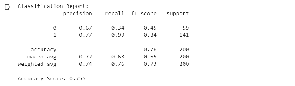
6.2 SVM
SVM stands for Support Vector Machine, and it is a popular supervised machine learning algorithm used for both classification and regression tasks.
In SVM, the main objective is to find the optimal hyperplane that best separates data points of different classes in a high-dimensional feature space. The hyperplane is a decision boundary that maximizes the margin, which is the distance between the closest data points (support vectors) of different classes. SVM aims to achieve the largest margin to enhance the model's ability to generalize well to new, unseen data.
The key features of SVM are:
-
Linear Separability: SVM is particularly effective when the data points are linearly separable, meaning they can be separated by a straight line (in 2D), plane (in 3D), or hyperplane (in higher dimensions).
-
Kernel Trick: SVM can handle non-linearly separable data by using the "kernel trick." It transforms the original feature space into a higher-dimensional space where the data points may become linearly separable. Common kernel functions include Polynomial, Gaussian (RBF), and Sigmoid kernels.
-
Margin and Regularization: SVM has a regularization parameter (C) that controls the trade-off between maximizing the margin and minimizing the classification error on the training data. A larger C value allows for a smaller margin and may result in some misclassifications on the training data, while a smaller C value leads to a larger margin but might risk overfitting.
-
Multi-class Classification: SVM is a binary classifier, but it can be extended to handle multi-class classification tasks using methods like one-vs-one or one-vs-rest strategies.
SVM is known for its ability to handle high-dimensional data and its robustness against overfitting, especially in cases of limited training samples. However, for large datasets, SVM's training time and memory requirements can become a concern. In such cases, variants like Linear SVM or Stochastic Gradient Descent (SGD) SVM are often used to speed up training.
from sklearn.model_selection import GridSearchCV
from sklearn import svm
from sklearn.metrics import classification_report

# define the model
svc = svm.SVC()

# define the parameters for grid search
parameters = {'kernel': ('linear', 'rbf', 'poly'), 'C':[0.1, 1, 10], 'gamma':[1, 0.1, 0.01]}

# instantiate the grid search with 5-fold cross-validation
clf = GridSearchCV(svc, parameters, cv=5)

# fit the model to the training data
clf.fit(X_train, y_train)

# print the best hyperparameters
print("Best Parameters:\n", clf.best_params_)

# predict the test set results
y_pred = clf.predict(X_test)

# print the performance metrics
print(classification_report(y_test, y_pred))
Out: 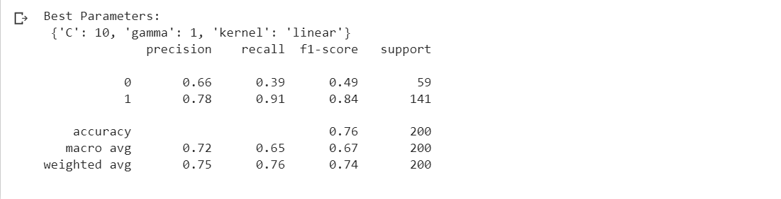
6.3 MLP
MLP stands for Multilayer Perceptron, and it is a type of artificial neural network used for both classification and regression tasks. MLP is a feedforward neural network, which means the information flows in one direction, from the input layer through the hidden layers to the output layer, without any feedback loops.
The architecture of an MLP consists of multiple layers of interconnected nodes or neurons. The network typically consists of three main types of layers:
-
Input Layer: This is the first layer that receives the raw input data. Each neuron in the input layer corresponds to a feature in the input data, and the number of neurons in this layer is determined by the dimensionality of the input data.
-
Hidden Layers: Between the input and output layers, there can be one or more hidden layers. Each hidden layer consists of multiple neurons, and these neurons are responsible for learning and extracting patterns and representations from the input data. The more hidden layers and neurons in each layer, the more complex patterns the network can learn.
-
Output Layer: The output layer produces the final predictions or results based on the learned representations from the hidden layers. The number of neurons in the output layer depends on the nature of the task. For example, in binary classification, there will be one neuron for each class, whereas in multi-class classification, there will be multiple neurons, one for each class.
MLP uses a process called forward propagation to compute the outputs. The input data is fed into the input layer, and the information passes through the hidden layers with each neuron performing a weighted sum of its inputs, followed by a non-linear activation function. The activation function introduces non-linearity to the network, allowing it to learn complex relationships in the data.
During training, MLP uses an optimization algorithm (usually gradient descent or its variants) to update the weights of the neurons, minimizing the difference between the predicted outputs and the actual labels (i.e., the loss function). This process is known as backpropagation, where the error is propagated backward through the network to adjust the weights and improve the model's performance.
MLP is a powerful and flexible model capable of learning complex patterns in data, but it requires careful tuning of hyperparameters such as the number of hidden layers, the number of neurons per layer, learning rate, and the choice of activation functions. Additionally, training an MLP can be computationally intensive, especially for large datasets and complex architectures. However, with the advancement of hardware and optimization techniques, MLP has become a widely used and effective tool in various machine learning applications, including image recognition, natural language processing, and more.
from sklearn.model_selection import GridSearchCV
from sklearn.neural_network import MLPClassifier
from sklearn.metrics import classification_report
from sklearn.preprocessing import StandardScaler

mlp = MLPClassifier(max_iter=1000)

parameter_space = {
    'hidden_layer_sizes': [(50,50,50), (50,100,50), (100,)],
    'activation': ['tanh', 'relu'],
    'solver': ['sgd', 'adam'],
}

clf = GridSearchCV(mlp, parameter_space, n_jobs=-1, cv=5)
clf.fit(X_train, y_train)

print('Best parameters found:\n', clf.best_params_)

final_mlp = MLPClassifier(max_iter=1000, **clf.best_params_)
final_mlp.fit(X, y)

y_pred = final_mlp.predict(X_test)
print(classification_report(y_test, y_pred))
Out: 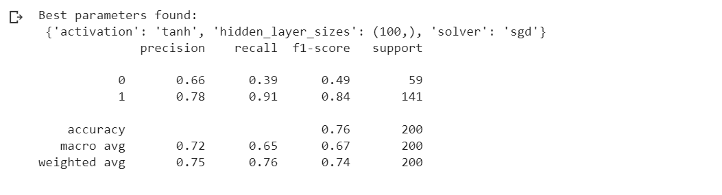
6.4 Logistic Regression
Logistic Regression is a popular and widely used binary classification algorithm in machine learning. Despite its name, it is primarily used for classification tasks rather than regression. The fundamental idea behind logistic regression is to model the probability of an input belonging to a particular class.
In binary classification, the output of logistic regression is a probability score between 0 and 1, representing the likelihood of the input belonging to one of the two classes (e.g., "positive" or "negative," "yes" or "no"). The predicted probability is then compared to a threshold (typically 0.5), and the input is assigned to the class with the higher probability.
The key components of logistic regression are as follows:
- Sigmoid (Logistic) Function: The core of logistic regression is the sigmoid function, also known as the logistic function. It maps any real-valued number to a value between 0 and 1. The sigmoid function is expressed as:
sigmoid(z) = 1 / (1 + exp(-z))
where 'z' is the linear combination of input features and their corresponding weights.
-
Linear Model: In logistic regression, a linear model is used to combine the input features with their respective weights. The linear combination is then passed through the sigmoid function to obtain the predicted probability.
-
Decision Boundary: The decision boundary is a threshold that determines how the predicted probabilities are mapped to class labels. For example, if the threshold is set to 0.5, any predicted probability greater than or equal to 0.5 will be assigned to one class, and any probability less than 0.5 will be assigned to the other class.
-
Training: During training, logistic regression optimizes its weights to minimize a cost function, such as the cross-entropy or log-loss. The cost function quantifies the difference between the predicted probabilities and the actual class labels.
Logistic regression is a linear model, which means it can only learn linear decision boundaries between classes. However, by using polynomial or interaction terms, it can be extended to capture non-linear relationships. Moreover, logistic regression is computationally efficient and relatively easy to interpret, making it a popular choice for binary classification tasks.
Though logistic regression is commonly used for binary classification, it can also be extended to handle multi-class classification problems using techniques like one-vs-rest or multinomial logistic regression. Overall, logistic regression is a powerful and interpretable algorithm that serves as a fundamental building block in many machine learning applications.
from sklearn.linear_model import LogisticRegression
from sklearn.model_selection import GridSearchCV

# setup the hyperparameter grid
param_grid = [
    {'penalty': ['l1'], 'solver': ['liblinear', 'saga'], 'C': [0.001, 0.01, 0.1, 1, 10, 100]},
    {'penalty': ['l2'], 'solver': ['newton-cg', 'lbfgs', 'sag', 'saga', 'liblinear'], 'C': [0.001, 0.01, 0.1, 1, 10, 100]},
    {'penalty': ['elasticnet'], 'solver': ['saga'], 'l1_ratio': [0.5], 'C': [0.001, 0.01, 0.1, 1, 10, 100]},
    {'penalty': ['none'], 'solver': ['newton-cg', 'lbfgs', 'sag', 'saga']}
]

# instantiate the logistic regression model
logreg = LogisticRegression()

# instantiate the grid search model
grid_search = GridSearchCV(estimator=logreg, param_grid=param_grid, cv=5, n_jobs=-1)

# fit the grid search to the data
grid_search.fit(X_train, y_train)

# print the best parameters
print("Best Parameters: ", grid_search.best_params_)

# instantiate the logistic regression model with best parameters
best_logreg = LogisticRegression(C=grid_search.best_params_['C'], penalty=grid_search.best_params_['penalty'], solver=grid_search.best_params_['solver'])

# fit the model with the training data
best_logreg.fit(X_train, y_train)

# make predictions on the test data
y_pred = best_logreg.predict(X_test)

# evaluate the model
from sklearn.metrics import classification_report, accuracy_score
print("Accuracy: ", accuracy_score(y_test, y_pred))
print(classification_report(y_test, y_pred))
Out: 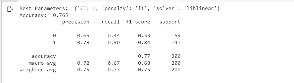
6.5 Decision Tree
A Decision Tree Classifier is a powerful and intuitive machine learning algorithm used for both classification and regression tasks. It is a non-linear model that partitions the data into subsets based on a series of binary decisions. Each decision corresponds to a node in the tree, and the data is split based on specific features and their corresponding thresholds.
The key features of a Decision Tree Classifier are as follows:
-
Recursive Binary Splitting: The decision tree builds a tree structure through recursive binary splitting. It starts at the root node, which represents the entire dataset. The algorithm selects the best feature and threshold to split the data into two subsets at each node, with the goal of maximizing the homogeneity or purity of the subsets. This process is repeated for each child node until certain stopping criteria are met.
-
Entropy and Information Gain: Decision trees commonly use metrics like entropy and information gain to measure the homogeneity of a node. Entropy quantifies the impurity or disorder in the node's class distribution, while information gain represents the reduction in entropy achieved by splitting the data based on a particular feature. The algorithm chooses the feature that results in the highest information gain for each split.
-
Leaf Nodes and Decision Rules: The terminal nodes of the tree are called leaf nodes. Each leaf node corresponds to a class label in the case of classification tasks or a target value in regression tasks. The decision rules along the path from the root to a specific leaf node provide the decision-making process for predicting the class or target value of a new data point.
-
Overfitting: Decision trees have the tendency to create overly complex trees that perfectly fit the training data, leading to overfitting. To mitigate this, techniques like pruning, limiting the tree depth, or setting a minimum number of samples per leaf node are used to prevent excessive branching.
Decision trees are highly interpretable, as the decision-making process is transparent and easy to visualize. However, they may not generalize well to unseen data when the tree becomes too deep and complex. To address this limitation, ensemble methods like Random Forest and Gradient Boosting, which combine multiple decision trees, are often used to improve accuracy and robustness.
Decision Tree Classifiers are widely used in various domains due to their simplicity, effectiveness, and interpretability. They are particularly well-suited for datasets with non-linear relationships and categorical features, making them a versatile tool in machine learning applications such as customer churn prediction, medical diagnosis, and sentiment analysis, among others.
# Import the required packages
from sklearn.model_selection import GridSearchCV
from sklearn.tree import DecisionTreeClassifier
from sklearn.metrics import accuracy_score, classification_report

# Define the parameter grid
param_grid = {
    'max_depth': [3, 5, 10, 20],
    'min_samples_split': [2, 5, 10],
    'min_samples_leaf': [1, 2, 5]
}

# Instantiate the classifier
dtree = DecisionTreeClassifier(random_state=42)

# Instantiate the GridSearchCV object
grid_search = GridSearchCV(dtree, param_grid, cv=5)

# Fit the model
grid_search.fit(X_train, y_train)

# Get the best parameters
best_params = grid_search.best_params_
print("Best parameters: ", best_params)

# Train the final model with the best parameters
final_model = DecisionTreeClassifier(**best_params)
final_model.fit(X_train, y_train)

# Predict the labels of the test set
y_pred = final_model.predict(X_test)

# Print the accuracy score and classification report
print("Accuracy: ", accuracy_score(y_test, y_pred))
print(classification_report(y_test, y_pred))
Out: 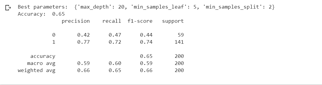
Conclusion based on classification reports
- KNN
- SVM
- MLP
- Logistic Regression
- Decision Tree
- KNN:
- The model shows a relatively higher recall (0.93) for class 1, indicating that it can effectively identify positive cases.
- However, the precision for class 0 (0.67) is lower, suggesting that it struggles in correctly predicting negative cases.
- The F1-score for class 1 is high (0.84), indicating a good balance between precision and recall for positive cases.
- The overall accuracy of the model is 0.755.
- SVM:
- Similar to the Multilayer Perceptron, the SVM model shows a high recall (0.91) for class 1, indicating its ability to identify positive cases effectively.
- The precision for class 0 (0.66) is relatively lower, suggesting challenges in accurately predicting negative cases.
- The F1-score for class 1 is high (0.84), indicating a good balance between precision and recall for positive cases.
- The overall accuracy of the model is 0.76.
- Multilayer Perceptron:
- The model exhibits a high recall (0.91) for class 1, indicating its capability to identify positive cases effectively.
- However, the precision for class 0 (0.66) is relatively lower, suggesting it struggles in accurately predicting negative cases.
- The F1-score for class 1 is high (0.84), indicating a good balance between precision and recall for positive cases.
- The overall accuracy of the model is 0.76.
- Logistic Regression:
- The model demonstrates a high recall (0.90) for class 1, indicating its effectiveness in correctly predicting positive cases.
- The precision for class 0 (0.65) is relatively low, suggesting a lower ability to predict negative cases accurately.
- The F1-score for class 1 is high (0.84), indicating a good balance between precision and recall for positive cases.
- The overall accuracy of the model is 0.765.
- Decision Tree:
- The model's precision for both classes is moderate, with class 1 having higher precision (0.77).
- The recall for class 1 (0.72) suggests that the model performs reasonably well in identifying positive cases, but it's lower for class 0 (0.47).
- The F1-score for class 1 is higher (0.74) than class 0 (0.44).
- The overall accuracy of the model is 0.65.
Overall, the Logistic Regression, Multilayer Perceptron, and SVM models seem to perform relatively better compared to KNN and Decision Tree. They exhibit higher recall for class 1 and better overall accuracy. However, the choice of the best model depends on the specific requirements and objectives of the task. If the ability to correctly identify positive cases (higher recall for class 1) is crucial, then Logistic Regression, Multilayer Perceptron, or SVM might be preferred. If interpretability is a priority, Logistic Regression could be a suitable option.