Reading time: 30 minutes

What are Autoencoders?

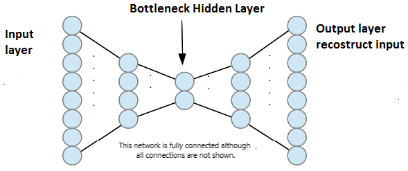
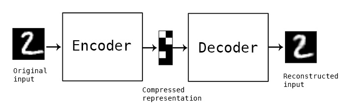
Autoencoders are a type of unsupervised neural networks. Here, the number of neurons in the output layer and the input layer is the same i.e the output and the input of this neural network is nearly the same.

Why are they used?

As we all know, neural networks contain an internal representation of the input in each of it's hidden layer. One of the hidden layers of the autoencoder, has lesser number of neurons as compared to other layers. This layer is called 'bottleneck' layer. The number of neurons in this layer is much lesser than that in input layer, so the data represented in this layer is a compressed version of the data represented at the input layer. This concept where we compress the data, is also known as dimensionality reduction. Autoencoders are used to get this compressed data.

Key points about Autoencoders

1. Autoencoders are data-specific, which means that they will only be able to compress data similar to what they have been trained on.
2. Autoencoders are lossy, which means that the decompressed outputs will be degraded compared to the original inputs.
3. Autoencoders are learned automatically from data examples, which is a useful property: it means that it is easy to train specialized instances of the algorithm that will perform well on a specific type of input. It doesn't require any new engineering, just appropriate training data.

What are Autoencoders used for?

Mostly, autoencoders are used for :

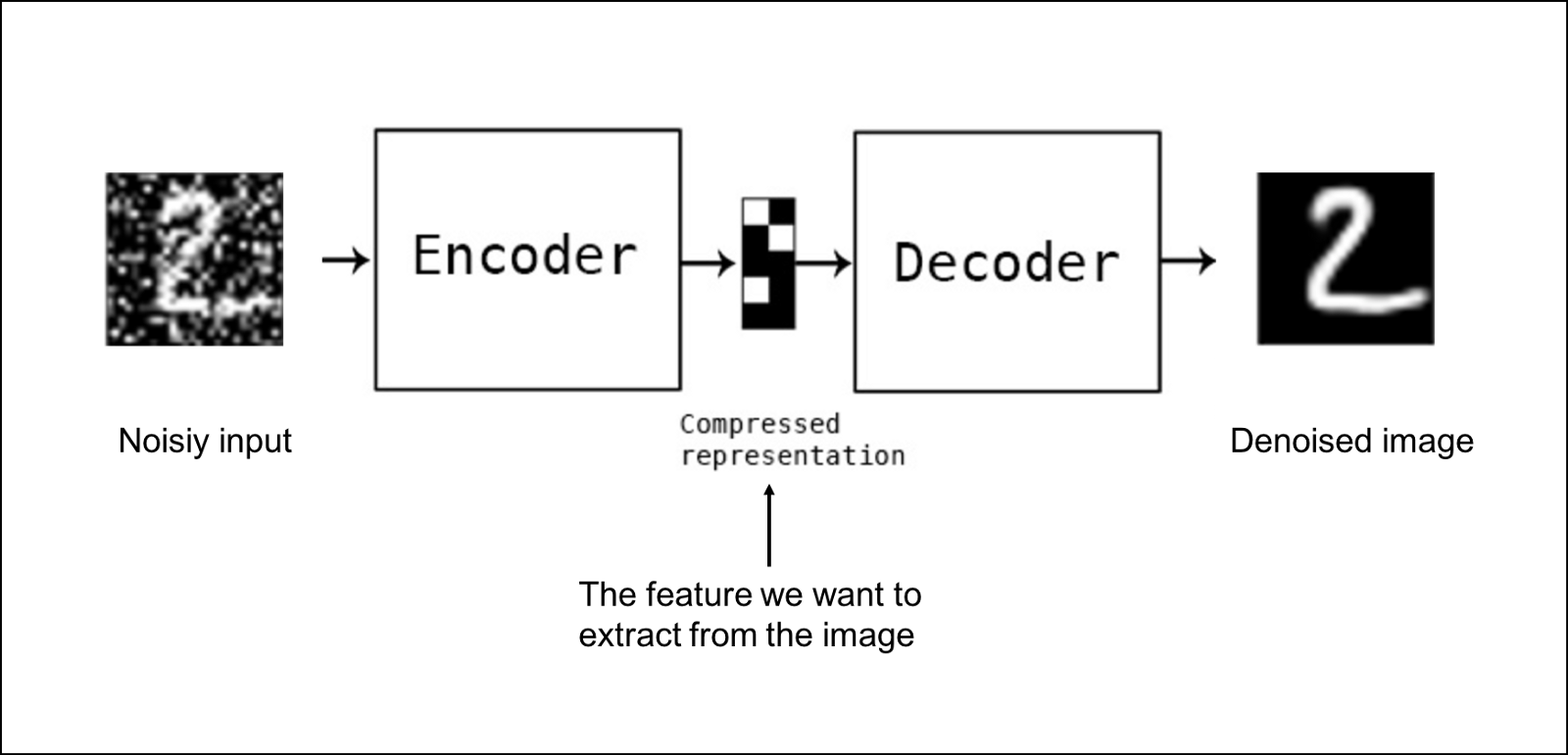
1. Data denoising : Here, the autoencoders are used to reconstruct the input from a corrupted version of it.

2. Dimensionality reduction for data visualization : For 2D visualization specifically, t-SNE (pronounced "tee-snee") is probably the best algorithm around, but it typically requires relatively low-dimensional data. So a good strategy for visualizing similarity relationships in high-dimensional data is to start by using an autoencoder to compress your data into a low-dimensional space (e.g. 32 dimensional), then use t-SNE for mapping the compressed data to a 2D plane. Note that a nice parametric implementation of t-SNE in Keras was developed by Kyle McDonald and is available on Github. Otherwise scikit-learn also has a simple and practical implementation.

Now let's build a simple autoencoder using tensorflow !

import numpy as np 
import pandas as pd  
import math  
#Input data files are available in the "../input/" directory.
#For example, running the next statement will list the files in the input directory
import os
print(os.listdir("../input"))
import matplotlib.pyplot as plt
import tensorflow as tf
from tensorflow.contrib.layers import fully_connected

We have started by importing the libraries and frameworks required. numpy is used for linear alzebra; pandas for data processing, CSV file I/O (e.g. pd.read_csv); math for using mathematical functions like round(), sin) etc; os to keep track of the input and output files in the directory specified; matplotlib for plotting and tensorflow for building our model.

training_data = pd.read_csv("../input/train.csv")
train_data = (training_data.iloc[0:math.floor(len(training_data.index)*0.7),1:].values, training_data.iloc[0:math.floor(len(training_data.index)*0.7),0].values)
test_data = (training_data.iloc[math.floor(len(training_data.index)*0.7)+1:,1:].values, training_data.iloc[math.floor(len(training_data.index)*0.7)+1:,0].values)

Here, we imported the dataset in the directory "../input". The file we imported was in CSV format. Then we divided it into training (70 %) and testing dataset (30 %). The dataset we used is the MNIST dataset available here.

tf.reset_default_graph() # Clears the default graph stack and resets the global default graph
batch_size = tf.placeholder(tf.int64)
num_features =  len(training_data.columns)-1
X = tf.placeholder(tf.float32, shape=[None, num_features])
training_dataset = tf.data.Dataset.from_tensor_slices( X ).batch(batch_size).repeat()
iter1 = training_dataset.make_initializable_iterator()
features = iter1.get_next()

Here, we created a placeholder for the batch size. The placeholder is like a declaration of a tensor variable which you can initialize later. Batch size is the number of training examples you want to give as an input to the model at a time.
A very important point to note here is that using feed-dict, is the slowest way to input data in your model. It must be avoided. For that, Tensorflow has a built-in API, Dataset, which makes it very easy to do. In this article, as a bonus ;) , you'll learn to use Dataset API to create an Input Pipeline so that the GPU has to never wait for the next stuff to come in. For detailed information on built-in pipelines, have a look at this amazing article here.

input_features = 784 #28x28 pixels
hidden_units1 = 392
hidden_units2 = 196
hidden_units3 = 98
hidden_units4 = hidden_units2
hidden_units5 = hidden_units1
output_units = input_features

learning_rate = 0.01

actf = tf.nn.relu

Here, we define the number of units in each layer, learning rate and the activation function to be used. All of this defines the basic structure of the Tensorflow graph. Tensorflow graph is actually the core of everything. The graph consists of nodes which perform some operation on the data coming in to it in the form of a data structure called tensor. Several such nodes are connected to each other to create a complete model.

initializer = tf.variance_scaling_initializer() #this is done to make the variance of the outputs equla to that of variance of inputs

wt1 = tf.Variable(initializer([input_features, hidden_units1]), dtype = tf.float32)
wt2 = tf.Variable(initializer([hidden_units1, hidden_units2]), dtype = tf.float32)
wt3 = tf.Variable(initializer([hidden_units2, hidden_units3]), dtype = tf.float32)
wt4 = tf.Variable(initializer([hidden_units3, hidden_units4]), dtype = tf.float32)
wt5 = tf.Variable(initializer([hidden_units4, hidden_units5]), dtype = tf.float32)
wt6 = tf.Variable(initializer([hidden_units5, output_units]), dtype = tf.float32)

b1 = tf.Variable(tf.zeros(hidden_units1))
b2 = tf.Variable(tf.zeros(hidden_units2))
b3 = tf.Variable(tf.zeros(hidden_units3))
b4 = tf.Variable(tf.zeros(hidden_units4))
b5 = tf.Variable(tf.zeros(hidden_units5))
b6 = tf.Variable(tf.zeros(output_units))

Here, we defined the weights and biases to be used in our model.

hidden_units1 = actf(tf.matmul(features,wt1)+b1)
hidden_units2 = actf(tf.matmul(hidden_units1,wt2)+b2)
hidden_units3 = actf(tf.matmul(hidden_units2,wt3)+b3)
hidden_units4 = actf(tf.matmul(hidden_units3,wt4)+b4)
hidden_units5 = actf(tf.matmul(hidden_units4,wt5)+b5)
output_units = actf(tf.matmul(hidden_units5,wt6)+b6)

Here, we defined the feed-forward mechanism in our model. We can get a quick look at the math behind this autoencoder too. Here is the formula used above :
$$A_l = A.F.(Z_{l-1}*W_{l-1} + b_{l-1} )$$
where, $A_l$ is the activation unit of $l^{th}$ layer
$A.F.$ is the activation function used (in our case, we are using ReLU or Rectified Linear Unit activation function)
$Z_{l-1}$ is the input coming from the $(l-1)^{th}$ or the previous layer
$W_{l-1}$ are the weights of $(l-1)^{th}$ layer and
$b_{l-1}$ is the bias unit of $(l-1)^{th}$ layer

The weights and biases are initialised with random values in the upcoming part of the code. Here, we have defined how exactly we are going to use those weights and biases. We start with the inputs given to the first layer and calculate the activation units of next layer which becomes the input to the layer after it and so on and so forth until we get the output units. Then comes the role of loss function which tell us how much error is there in our current output units.

loss = tf.reduce_mean(tf.square(output_units - features))

Defined the loss (also calles reconstruction error here) function here. The formula used is :
$$loss = \frac{\sum_{i=0}^n (OutputUnit - InputUnit)^2}{n}$$
where, $n$ is the number of units in output and input layer (both have same in case of autoencoder as we have seen already)

optimizer = tf.train.AdamOptimizer()
train = optimizer.minimize(loss)optimizer = tf.train.AdamOptimizer()
train = optimizer.minimize(loss)

Defined the optimizing function. This is where the actual learning happens. The optimizing function defines how we are going to update our parameters (weights and biases) in order to reduce the reconstruction error. Backpropagation comes into play here. It is based on the famous chain rule of differentiation. It starts with the reconstruction error and propagates this error in the backward direction towards the input features (hence the name "back"-propagation). As it moves backwards, it keeps updating the weights and biases in each layer. Once the updation is done, the feed-forward mechanism takes place again, and this time the reconstruction error will be a little reduced (cuz our model has "learnt" a little bit about the network, inputs and required outputs !). Again the backpropagation occurs and so on so forth until the number of iterations to be done is finished or the reconstruction error falls below a certain specified value.

init = tf.global_variables_initializer()

epoch_num = 5
BATCH_SIZE = 150
num_test_images = 10
num_batches = math.floor(training_data.shape[0]*0.7)//BATCH_SIZE

Here, we defined the number of epochs. It is the number of times we will go give batches to the model for training.Usually, it is defined as the number of times, we will go through the entire dataset but here I have a created an input pipeline in such a way that it will care of providing the data no matter how many times we request for a batch input. So all we need here is to tell it how many number of times we will need a batch of the dataset.
We also defined the batch size, number of test images, we will use to visualize and the number of unique batches in our training dataset.

with tf.Session() as sess:
    sess.run(init)
    sess.run(iter1.initializer, feed_dict={ X: train_data[0], batch_size: BATCH_SIZE})
    print('Training...')
    for epoch in range(epoch_num):
        print(epoch)
        tot_loss = 0
        for _ in range(num_batches):
            _, loss_value = sess.run([train, loss])
            tot_loss += loss_value
        print("Iter: {}, Loss: {:.4f}".format(epoch, tot_loss / num_batches))
    
    # initialise iterator with test data
    sess.run(iter1.initializer, feed_dict={ X: test_data[0], batch_size: num_test_images})
    results = sess.run(output_units)
    
    #let us see how the constructions look like
    f, a = plt.subplots(2,10,figsize=(20,4))
    for i in range(10):
        a[0][i].imshow(np.reshape(test_data[0][i],(28,28)))
        a[1][i].imshow(np.reshape(results[i],(28,28)))

Here, we executed the graph we have defined earlier. The compressed data or the hidden features that we wanted to extract from the image are stored in "hidden_units3" tensor which can be used later on. Also, let us take a look at the output images (the reconstructed images).

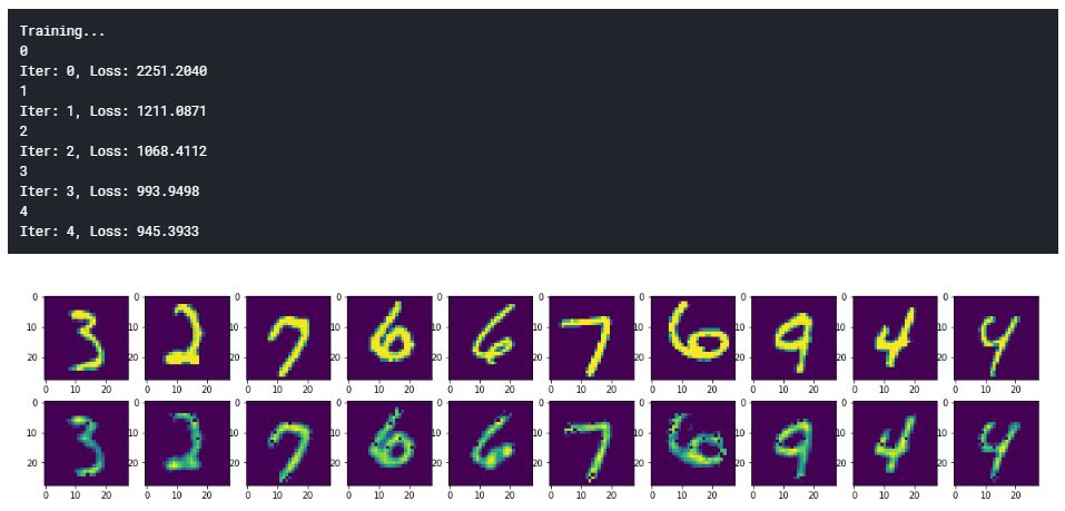
As we can see, we trained only on 5 batches, which is less than 10 % of the entire dataset. But still the reconstructed images look so similar. That's the power of neural networks!! You can increase the number of batches to any value you like, (keeping in mind, it will take a longer time :p ) and reduce the reconstruction error. Hope you enjoyed this article. The entire code is github.com/pratap-is-here/Autoencoder-using-tensorflow. Thanks.