Kohonen Neural Network

Introduction

The Kohonen Neural Network (KNN) also known as self organizing maps is a type of unsupervised artificial neural network. This network can be used for clustering analysis and visualization of high-dimension data.

It involves ordered mapping where input data are set on a grid, usually 2 dimensional. It reduces dimensionality of inputs by mapping its input to a simpler version of itself while preserving its underlying structure. The key characteristic of KNN is that its self organizing, where nodes are grouping themselves based on the features of the input data.

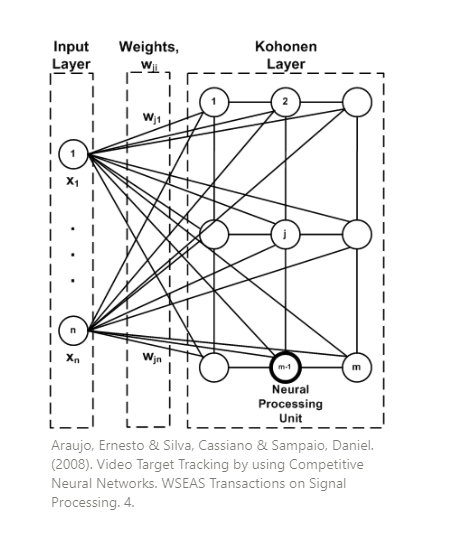
Another way to look into it is like having layers, the input and output layer, and the basic units are neurons. The input neurons are connected to the output neurons and they have weights. The input layer recieves the input data and the values are sent to the output layer. The output neuron with the strongest response will be the winnerand answer for the input data.

How it works

The components of the network are the weight and the input vectors. Each weight is initialized in the beginning, this has the same dimensionality as the input data. Weights also have a natural location, this will tell its x,y location in the 2D map.

The algorithm works as follows:

1. The first step is to initialize the weights randomly or you can randomly choose examples from the training set. In this example we will use random iteration.
   
   

2. After initializing the weights we now randomly select an input and get the Best Matching Unit (BMU). We can call BMU as the competition winner because it’s the weight that is closest to the input. The method to compute for the BMU is using the Euclidean distance. The weight with the smallest distance will have their position slightly adjusted to match the input. The equation for BMU is:
   
   
   $inputDistance^2 = \overset{i=n}{\underset{i=0}{\sum}} ( I_i - W_i)^2$
   
   
   where:
   I = current input
   W = node’s weight
   n = number of weights
   
   

3. After getting the BMU its weight vector will be updated and so is its neighboring weights. The radius of the neighborhood of the BMU is also calculated. Any nodes found within the radius of the BMU will be adjusted to make it close to the input vector. The closer a node is to the BMU, the more its' weights are altered. The formula for the wight update is as follows:
   
   
   Weight update formula: $\triangle w_{j,i} = n(t) * T_{j,I(x)}(t)*(x_i-w_{j,i})$
   
   where:
   t=epoch
   i = weight/neuron
   j = another weight/neuron
   I(x) = BMU / winning neuron
   
   

Where:
Learning Rate = $n(t) = \eta_0 exp(-\frac {t}{\tau_\eta})$
Depends on epoch, as epoch rise learning rate decreases. overtime the weights update less and converge to a value

Topological Neighborhood = $S_{j,i} = ||w_j - w_i ||$
Depends on distance of neurons and neighborhood size.

Lateral distance between neurons = $\sigma (t) = \sigma _ 0exp(-\frac {t}{\tau_0})$

Neighborhood = $\sigma (t) = \sigma _ 0exp(-\frac {t}{\tau_0})$
This is for calculating the size of the neighborhood around the BMU

4. Repeat the steps again from step 2 using a different input

Pseudo code

• Initialize the value of the weight
• Repeat until convergence or maximum epochs are reached
  • select randomly a value from the training set
  • For each input instance x
    • Find the best matching unit BMU
    • Update the weight vector of BMU and its neighboring cells

Code implementation

import math
import numpy as np
import matplotlib.pyplot as plt

def BMU(SOM,x):
    distSq = (np.square(SOM - x)).sum(axis=2)
    return np.unravel_index(np.argmin(distSq, axis=None), distSq.shape)

def update_weights(SOM, train_ex, learn_rate, radius_sq, 
                   BMU_coord, step=3):
    g, h = BMU_coord
    
    if radius_sq < 1e-3:
        SOM[g,h,:] += learn_rate * (train_ex - SOM[g,h,:])
        return SOM
    # Change all cells in a small neighborhood of BMU
    for i in range(max(0, g-step), min(SOM.shape[0], g+step)):
        for j in range(max(0, h-step), min(SOM.shape[1], h+step)):
            dist_sq = np.square(i - g) + np.square(j - h)
            dist_func = np.exp(-dist_sq / 2 / radius_sq)
            SOM[i,j,:] += learn_rate * dist_func * (train_ex - SOM[i,j,:])   
    return SOM    


def train_SOM(SOM, train_data, learn_rate = .1, radius_sq = 1, 
             lr_decay = .1, radius_decay = .1, epochs = 10):    
    learn_rate_0 = learn_rate
    radius_0 = radius_sq
    for epoch in np.arange(0, epochs):
        rand.shuffle(train_data)      
        for train_ex in train_data:
            g, h = BMU(SOM, train_ex)
            SOM = update_weights(SOM, train_ex, 
                                 learn_rate, radius_sq, (g,h))
        
        learn_rate = learn_rate_0 * np.exp(-epoch * lr_decay)
        radius_sq = radius_0 * np.exp(-epoch * radius_decay)            
    return SOM


if __name__ == "__main__":
    
    #dimension of the grid 
    m, n = 10 , 10
    rand = np.random.RandomState(0)
    #initialize the inputs / training set
    #we will be using RGB colors
    x = 1000 # size of training set
    train_data = rand.randint(0, 255, (x, 3))
    
    SOM = rand.randint(0, 255, (m, n, 3)).astype(float)
    
    fig, ax = plt.subplots(
    nrows=1, ncols=4, figsize=(15, 3.5), 
    subplot_kw=dict(xticks=[], yticks=[]))
    total_epochs = 0

    for epochs, i in zip([1, 4, 5, 10], range(0,4)):
        total_epochs += epochs
        SOM = train_SOM(SOM, train_data, epochs=epochs)
        ax[i].imshow(SOM.astype(int))
        ax[i].title.set_text('Epochs = ' + str(total_epochs))

Output:




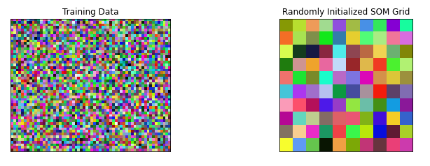
This is the initialized data visualized in a grid.




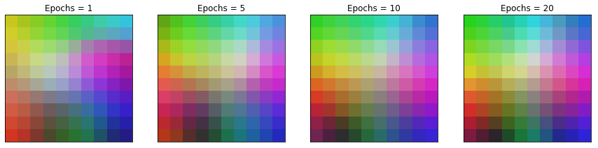
After using KNN it can be seen how from different epochs you can see how it arranges the RGB colors. AFter 10 epochs there is not much difference anymore.

Complexity

Time Complexity = $\mathcal{O}(NC)=\mathcal{O}(S^2)$

Where:
N = input vector size
C = number of cycles.
S = sample size

Applications

1. Speech Recognition Analysis
   Some studies implement KNN to create a representation of the spectre of speech samples. The different spectres are mapped to different parts of the map. The maps can be used for speech recognition systems.
   
   
2. Object Recognition
   KNN has also been used for dynamic object recognition. In SOM based object recognition weight updating and thresholding are the key issues being solved where each pixel is filtered as the foreground or background. You can read the st udy here
   
   
3. Interpretation o f EEG data
   KNN has also bee used in analyzing EEG data for emotion recognition. Features from EEG signals are classified and KNN is used to identify the boundaries of the EEG features.
   
   
   
   Sources:

• Yorek, Nurettin & Ugulu, Ilker & Aydin, Halil. (2017). kohonen-self-organizing-maps-shyam-guthikonda.
• Roussinov, H. $ Chen, D. A Scalable Self-organizing Map Algorithm (n.d.).
• for Textual Classification: A Neural Network Approach to Thesaurus Generation.
• IBM (2018) Kohonen Node. Retrieved from: ibm.com/docs/it/spss-modeler/18.1.0?topic=models-kohonen-node
• Saaad, M. (n.d.). Self-Organizing Maps: Theory and Implementation in Python with NumPy.