In this article, we have demonstrated a project "face" where we find the set of faces when combined, resulting in face of person A. We do this using Machine Learning techniques like Principal Component Analysis, Face Reconstruction and much more.
- Codebase on GitHub: github.com/OpenGenus/face
- Published as a pip package face-recons
- Developed by: Srishti Guleria
It can be installed by running below command in the terminal :
pip install face-recons==0.0.1
After successfully installing the package, user can enter python interpreter and enter:
from face_recons import main
Following it they will enter the Default Mode of the application.
The default mode of the application is interactive mode which is user friendly. The other mode is Command Line Interface.
Code Flow of our Application :
The default mode of the application is interactive mode which is user friendly. The other mode is Command Line Interface. The idea behind this applicayion was to make face reconstruction easier to apply to user's selected data and experiment on it. We start our application by defining three modules, main.py, train.py and test.py.
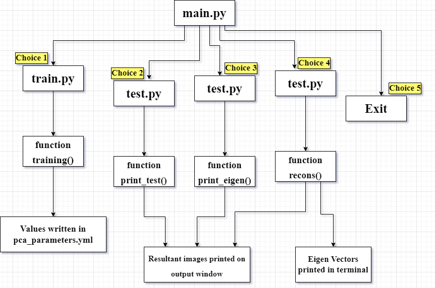
The application starts from main.py where we define our main menu. It contains the control code for our application since it controls execution of train.py & test.py.
Following it, functions from other python modules are called for performing the required tasks.
Default Mode (Interactive Mode):
Below diagram represents the Flow of Control of our application :
We start our application by opening the command prompt or terminal after installing the pip library. We start by typing below command in python interpreter :
from face_recons import main
Then following list shows up in the terminal :
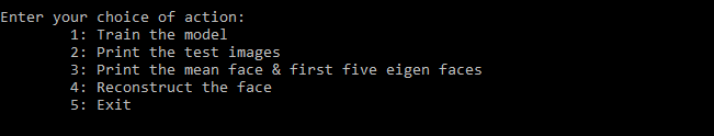
Choice 1
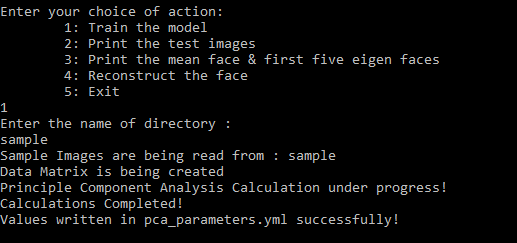
We can choose any option by entering 1 to 5. If we enter 1, then the model starts to train from images in the entered folder. The first step is generation of data matrix then the Principal Component Analysis gets calculated. After that the values are written in the pca_parameters.yml.
In our project, we would use the samples from the CalebA Dataset to train our model. For any image of 100 x 100 dimensions, it would have 100 x 100 x 3 numbers.
Hence, making a one dimensional array of thirty thousand elements.
def training():

    #we enter the directory name via main.py and read the images from that directory
	images = readImage(directory_name)

    #Save the size of images
	sz = images[0].shape

    #Create a data matrix
	data = matrix(images)
	print("Principle Component Analysis Calculation under progress! ", flush=True)

    #Eigen Vactor Calculations
    mean, eigenVectors = cv2.PCACompute(data, mean=None)
	print ("Calculations Completed!")

    #write them in pca_parameters.yml
	filename = "pca_parameters.yml"
	file = cv2.FileStorage(filename, cv2.FILE_STORAGE_WRITE)
	file.write("mean", mean)
	file.write("eigenVectors", eigenVectors)
	file.write("size", sz)
	file.release()
	print("Values written in pca_parameters.yml successfully!")
To calculate the eigen faces we would be required to perform following steps:
Firstly, we would get the Dataset containing the facial images. Then we would resize and adjust those images. Following it, we would create the matrix of data & then perform the PCA to calculate weights.
The calculation of weights would start by vectorizing the images, then subtracting the mean vectors. Following it we calculate the dot product of mean of vectors that have been subtracted with each principal component. Then we would multiply each weight to the Eigen Faces & resize and align the facial images to get the Eigen Faces via Eigen Vectors.
The training of model starts by calling the training() function from the train.py file. We start our python file by creating a directory referring to the folder containing the sample images. Then we would read those images and their size. Then we call the matrix function to accomplish our PCA calculations and the calculate the eigen vectors.
The training() function calls readImage(path) function. This function would read the sample images from our entered folder which contains sample images from the CalebA Dataset. We create an array of our images. We would list all points in the directory. Then we read all points from the text files. Then we add them to our array of images that we created. We convert our images to float values and add them to the list. Then we would flip the images and append them. If no images are found in the mentioned folder then an error message is returned.
Then the training() function calls matrix() function of train.py file to make data matrix. This function would create the data matrix for our sample images. Since each image has three colour channels : Red, Green and Blue, hence the space taken by an image would be equivalent to its height x width x 3.
Choice 2
If we choose choice 2, the collage of input/test images are printed on the output window. We are required to enter the full file path to test images.
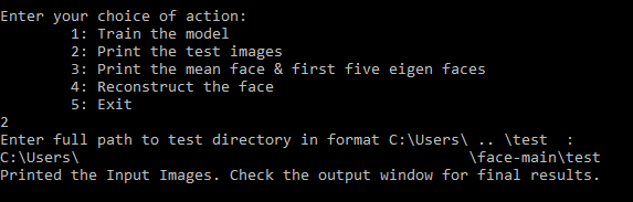
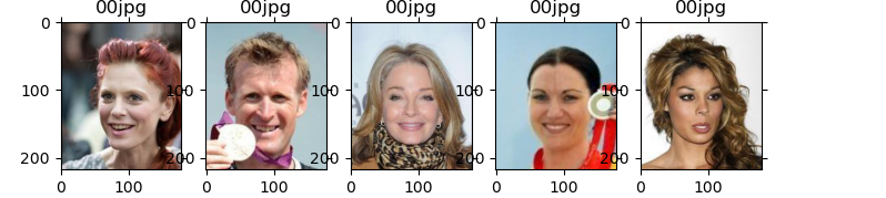
In this choice, the print_test() function of test.py file is called. We use matplotlib to print all images in the entered directory in form of collage by looping through them.
def print_test():
	#User inputs the dataset_path to enter directory
    dataset_path = input("Enter full path to test directory in format C:\\Users\\ .. \\test  : \n") + '/'

    #set height & width of images
	dataset_dir  = os.listdir(dataset_path)
	width  = 178
	height = 218
	test_image_names = dataset_dir
	testing_tensor   = np.ndarray(shape=(len(test_image_names), height*width), dtype=np.float64)

    # Print the test images by ploting on matplotlib
	print("Printed the Input Images. Check the output window for final results.\n")
	for i in range(len(test_image_names)):
		img = imread(dataset_path + test_image_names[i])
		plt.subplot(3,6,1+i)
		plt.title(test_image_names[i].split('.')[0][-2:]+test_image_names[i].split('.')[1])
		plt.imshow(img, cmap='gray')
		plt.subplots_adjust(right=1.000, top=1.000)
		plt.tick_params(labelleft='off', labelbottom='off', bottom='off',top='off',right='off',left='off', which='both')
	plt.show()
Choice 3
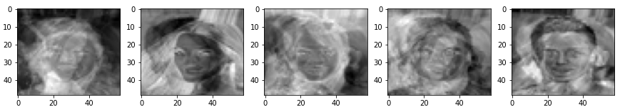
If we choose choice 3, then the mean face and first five eigen faces get printed on the output window one by one.
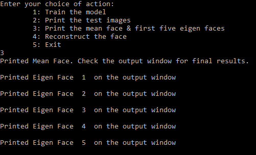
For this the print_eigen() function of test.py file is called. Here we first use matplotlib to loop through images and print the mean image in separate output window.
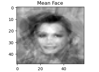
Then, using the same library we print 5 eigen faces in 5 separate output windows.
def print_eigen():

    #Enter path to 7 test images to print the mean & eigen faces

    neutral = []
	print('Enter path to 7 images below to produce mean face & eigen faces :\n')
	for i in range(7):
		i+=1
		p = input('Enter path to test image ' + str(i) + ' : \n')
		img = im.open(p).convert('L')
		img = img.resize((58,49), im.ANTIALIAS)

        #Vectorization of array
		img2 = np.array(img).flatten()
		neutral.append(img2)

	faces_matrix = np.vstack(neutral)
	mean_face = np.mean(faces_matrix, axis=0)

    #print the mean face
	plt.imshow(mean_face.reshape(49,58),cmap='gray');
	print('Printed Mean Face. Check the output window for final results.\n ')
	plt.title('Mean Face')
	plt.show()

    #print 5 eigen faces
    # normalization of faces matrix
	faces_norm = faces_matrix - mean_face
	faces_norm = faces_norm.T
	face_cov = np.cov(faces_norm)
	eigen_vecs, eigen_vals, _ = np.linalg.svd(faces_norm)

    # 5 Eigen Faces Visualization
	for i in np.arange(5):
		img = eigen_vecs[:,i].reshape(49,58)
		plt.imshow(img, cmap='gray')
		print('Printed Eigen Face ',i+1,' on the output window\n ')
		plt.title('Eigen Face :')
		plt.show()
Choice 4
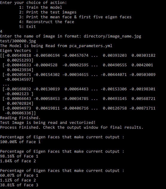
If we choose choice 4, then the trained model is read from pca_parameters.yml. The recons() function is called from the test.py file.
- Then the eigen vectors held in a structure of eigenVectors where eigen_face[i][j] = j-th eigen face of i-th image are displayed on the terminal as shown below.
- Then, the eigen faces will be read & obtained.
- Then we enter the name of image present in entered directory in format: directory/image_name.jpg. The image will be read and vectorized. After that the final results get displayed in new window. The final output window with original image on left and re-constructed image on right as described in the video below.
- Using reconstruction() function we could reconstruct our face of person A using the mean faces and Eigen Faces. As mentioned above we start by calculating the weights. The weights are the dot product of the mean image vactors that are subtracted with Eigen Vectors.
- Using disp() function we can display the original image against the reconstructed image as a result in new window.
- It has a slider for increasing or decreasing the number of eigen faces used for reconstruction. By trying all combinations, we can dynamically see the best reconstructed image.
- The reconstructed image dynamically changes with respect to the number of eigen faces chosen on slider.
- The percentage of Eigen Faces used for reconstructing output image is dynamically printed on the terminal as we move the slider.
def recons():
    #recons() function helps to reconstruct the faces with different number of eigen faces used
	def reconstruction(*args):
		final_output = average_face
        # We make percentage dict to store the weight of eigen face used
        # to reconstruct the current output
		percentage = {}
		for k in range(0,args[0]):
			weight = np.dot(imVector, eigenVectors[k])
			final_output = final_output + eigen_face[k] * weight
			#store weight in percentage dict
            percentage[k] = abs(weight)
        #display output
		disp(im, final_output)

        #Display the Percentage of Eigen Faces used for reconstruction dynamically
		total = 0
		if(len(percentage) > 0):
			print("\nPercentage of Eigen Faces that make current output :")
		for i in percentage:
			total = total + abs(percentage[i])
		for i in percentage:
			val = float(abs((percentage[i]/total)*100))
			if(val > 0 ):
				print(str("{:.2f}".format(val)) + "% of Face "+ str(i+1))


    #This function is used to display the Output Window
	def disp(x, y):
		final_output = np.hstack((x,y))
		final_output = cv2.resize(final_output, (0,0), fx=3, fy=3)
		cv2.imshow("Result", final_output)

    # Read the model from pcaparameters.yml
	model = "pca_parameters.yml"
	print("The Model is being Read from pca_parameters.yml", flush=True)
	file = cv2.FileStorage(model, cv2.FILE_STORAGE_READ)
	mean = file.getNode("mean").mat()

	eigenVectors = file.getNode("eigenVectors").mat()

    # show eigen vectors
	print("Eigen Vectors  :")
	print(eigenVectors)

    # Read eigen faces
	sz = file.getNode("size").mat()
	sz = (int(sz[0,0]), int(sz[1,0]), int(sz[2,0]))
	number_of_eigen_faces = eigenVectors.shape[0]
	print("Reading Finished.")
	average_face = mean.reshape(sz)

	eigen_face = []

    #obtain eigenfaces
	for eigenVector in eigenVectors:
		eigenFace = eigenVector.reshape(sz)
		eigen_face.append(eigenFace)


	# The test image is entered by user via main menu
	print("Test Image is being read and vectorized!")
	eigen_vec=[]
	im = cv2.imread(image_file)
	im = np.float32(im)/255.0
	imVector = im.flatten() - mean;
	eigen_vec.append(imVector)

    # Display output window
	print("Process Finished. Check the output window for final results.")
	final_output = average_face
	cv2.namedWindow("Result", cv2.WINDOW_AUTOSIZE)

    #change in the value of slider changes the number of eigen faces used for reconstruction
	cv2.createTrackbar("EigenFaces", "Result", 0, number_of_eigen_faces, reconstruction)

    #display test image on left & reconstructed image on right
	disp(im, final_output)
	cv2.waitKey(0)
	cv2.destroyAllWindows()
The output window contains the dynamic reconstructed image on the right as shown below :
Choice 5
Finally to exit the terminal we must enter 5. If we enter any other value than 1 to 5 then "invalid mode" output will be displayed.
Mode 1 (Command Line Interface)
If we wish to use the Command Line Interface, we can do so by typing the following command :
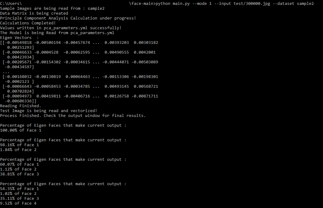
python main.py --mode 1 --input directory/image.jpg --dataset directory
We can enter mode = 1 for CLI mode, the directory/image.jpg for the Test Image and the directory for the Training Dataset.
- In the below example, we entered test/300000.jpg for Test Image and sample2 for Training Dataset.
- The model is trained from the pca_parameters.yml and the Test Image is reconstructed.
- The percentage of Eigen Faces used to reconstruct the output image is dynamically printed on terminal as we slide the slider.
- Same Output Window of Reconstructed Image is displayed in CLI mode as seen in Interactive Mode.
#We defined a parser for mode of interface. For enabling CLI, user would enter mode with value 1
parser.add_argument("--mode", default = False, help="Enable Command Line Interface", action='store')

#we defined input parser for getting the name of test image by user
parser.add_argument("--input", type=str, required=False, help="Enter the name of Test image in format: directory/image_name.jpg")

#we define the parser dataset to enter name of directory for training the model
parser.add_argument("--dataset", type=str,required=False, help="Enter the name of directory for Training the model")
Rest all code snippets for training and testing remain same as Interactive or Dafault Mode. The input image location and directory for training data entered via CLI are taken as input in this mode.