Radial Basis Function Neural Network (RBFNN) is one of the shallow yet very effective neural networks. It is widely used in Power Restoration Systems.

In this article we will discuss the following points:

1. What is an RBFNN ?
   

2. Radial Basis Function
   

3. Training an RBFNN
   

4. Solving the XOR problem using RBFNN
   

5. Similarities and differences with MLPs
   

6. Conclusion
   

1. What is an RBFNN ?

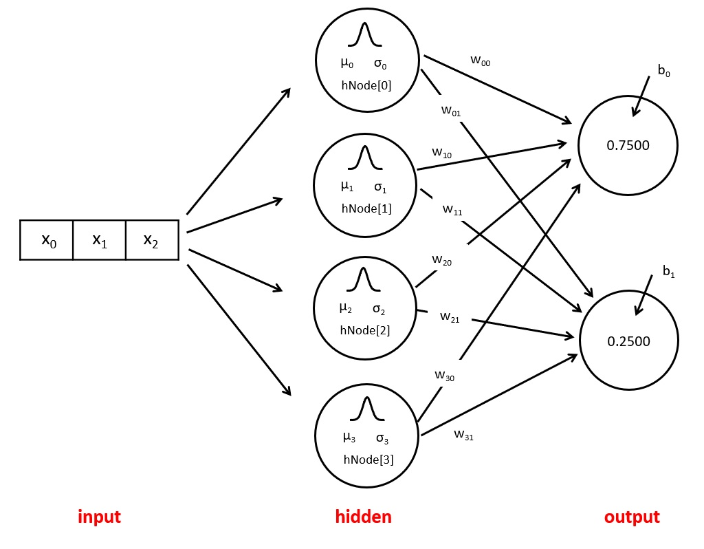
An RBFNN is a feed-forward neural network, composed from : an input layer representing the source of data, exactly one hidden layer with high dimension and an output layer to render the results of the network.

This type of neural networks is widely used in regression, function approximation and pattern classification problems.

Input Layer

Just like standard feed forward neural networks, the input layer is a one dimensional vector responsible for forwarding the data to the first hidden layer. Hence the number of neurons in this layer should be equal to the dimensionality of the data.

Hidden Layer

This layer is what makes RBFNN particular than standard Neural networks. Each neuron in this layer applies a non-linear activation function to its input, called Radial Basis Function (RBF), then forwards the results to the output layer.
The aim of this layer is to be able to separate the complex non-linear patterns in data in a more linear fashion. According to Cover's theorem on pattern separability

A complex pattern-classification problem, cast in a high-dimensional space non-linearly, is more likely to be linearly separable than in a low-dimensional space, provided that the space is not densely populated.

This means that a non-linear pattern in a law dimensional space is more likely to be separated linearly in a high dimensional space. Hence the number of neurons in this layer should be higher or equal to the number of neurons in the input layer.

Output Layer

Receives the results of the hidden layer and applies a linear activation function on them.

2. Radial Basis Function

In mathematics, a radial function is a function defined on an euclidean space Rn and whose value depends only on the distance between the input point and the origin.

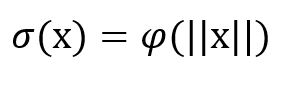
Therefore, each function that satisfies :

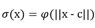
Where c is a point in Rn (called the center point) is also a radial function.

A collection of radial functions may form a basis for some function space of interest, hence the name "Radial Basis Function (RBF)".

One of the most used RBF in RBF networks is the Gaussian RBF. The standard Gaussian function is defined by the equation and the bell curve in the figure below :

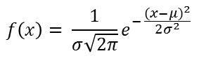
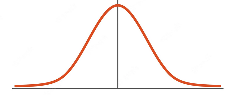
where :

• mu is the mean of the distribution and the center of the bell curve. It is called the prototype vector in RBF nets.
• sigma is the standard deviation.
• x is the input point.

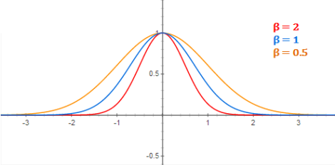
The Gaussian RBF activation is slightly different than the Gaussian function, it is defined by the following equation :

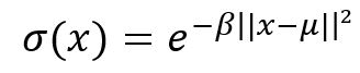
where beta is a hyper-parameter used to control the width of the bell curve as shown in the figure below:

3. Training radial basis network

In order to train an RBFNN, we need to define:

• The number of kernels to be used and the prototype vector for each neuron. Unsupervised learning techniques like kmean clustering are used to find the value of the prototype vectors.
• The weights between the hidden neurons and the output layer. This is done in a supervised manner by optimizing the least squares cost function.

4. Solving the XOR problem using RBFNN

In this section, we will first introduce the problem, then build the solution step by step.

Problem statement

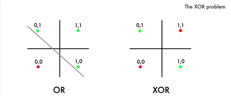
We want to predict the outputs of a XOR gate (exclusive or) using an artificial neural network. The figure below show the truth table of this binary gate.

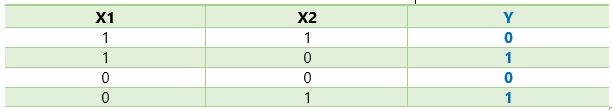
While single perceptron are known for their ability to predict the outputs of binary gates like OR and AND gates because they are linearly separable. The problem with the XOR gate is that her classes are not linearly separable like it is illustrated in the figure bellow. Hence we need to use a more complex network to solve the problem.

Solution

Radial basis networks are powerful ANNs used in approximation problems. Since classification problems are a special case of function approximation, where we are trying to approximate a score (0 or 1 ), RBF nets may then be usefull to solve the XOR problem.

In order to simplify our solution, we choose intuitively the number of radial kernels to be 2 and the center points for each RBF to be the fixed points : (0,1) and (1,0). With this being said, now we only need to find the weights between the hidden layer and the output layer using supervised-learning.

Let's first start by defining our class and its hyper-parameter

class RBFNN:
    
    def __init__(self, kernels,centers,beta=1,lr=0.1,epochs=80):
        
        self.kernels = kernels
        self.centers = centers
        self.beta = beta
        self.lr = lr
        self.epochs = epochs
        
        # Randomly initializes the weights and bias
        self.W = np.random.randn(kernels,1)
        self.b = np.random.randn(1,1)

• kernels: represents the number of RBFs to use which is also the number of neurons in the hidden layer.
• centers: is a vector containing the center of each RBF
• beta: is a hyper-parameter to control the width of the bell curve
• lr: learning rate
• epochs: number of training iterations.

RBF activation

We will use the gaussian RBF activation that has the following equation

    def rbf_activation(self,x,mu):
        return np.exp(-self.beta*np.linalg.norm(x - mu)**2)

This function is going to be used in the neurons of the hidden layer.

Linear activation (output)

The output layer uses a linear activation function, defined as follow :

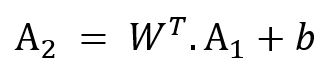
Where :

• W is the matrice of weights
• A1 is the vector having the RBF activations
• b is the bias

    def linear_activation(self,A):
        return self.W.T.dot(A) + self.b

Loss Function

The least square is a loss function usually used in regression problems, however when used in classification problems, the model tries to find a line or a hyper-plane to separate the data in two different regions which is the aim of our RBF network. If such a hyper-plane exists we say that the classes are linearly separable.

The equation of the least square loss is defined as follow :

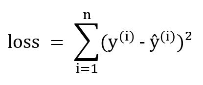
    def least_square_error(self,prediction,y):
        return (y - prediction).flatten()**2

Forward Propagation

    def _forward_propagation(self,x):
        # activations of the hidden layer
        a1 = np.array([
            [self.rbf_activation(x,center)] 
            for center in self.centers
        ])
        
        # activation of the output layer
        a2 = self.linear_activation(a1)
        
        return a2, a1

Back Propagation

The weights update rule in gradient descent is defined with the following equation :

Where :

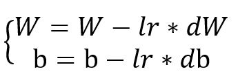
• dW is the derivative of the loss function relative to the weights.
• db is the derivative of the loss function relative to the bias.

We will not go through the details of the calculations, using the chain rule we will find the following equations:

Where :

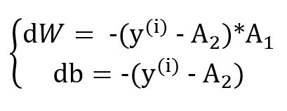
• A1 is the RBF activations (in the hidden layer).
• A2 is the linear activation (in the output layer).

    def _backpropagation(self, y, pred,a1):
        # gradients calculation
        dW = -(y - pred).flatten()*a1
        db = -(y - pred).flatten()
        
        # Weights update
        self.W = self.W -self.lr*dW
        self.b = self.b -self.lr*db
        
        return dW, db

Training Loop

    def fit(self,X,Y):
        
        for _ in range(self.epochs):
            
            for x,y in list(zip(X,Y)):
                # Forward propagation
                pred, a1 = self._forward_propagation(x)
                
                error = self.least_square_error(pred[0],y[0,np.newaxis])
                self.errors.append(error)
                
                # Back propagation
                dW, db = self._backpropagation(self,y,pred,a1)
                self.gradients.append((dW,db))

Prediction function

    def predict(self,x):
        a2,a1 = self._forward_propagation(x)
        
        return 1 if np.squeeze(a2) >= 0.5 else 0

Full code and execution results

import numpy as np


class RBFNN:
    
    def __init__(self, kernels,centers, beta=1,lr=0.1,epochs=80) -> None:
        
        self.kernels = kernels
        self.centers = centers
        self.beta = beta
        self.lr = lr
        self.epochs = epochs
        
        self.W = np.random.randn(kernels,1)
        self.b = np.random.randn(1,1)
        
        # to save the errors evolution
        # in case we want to check them later
        self.errors = []
        
        # to save the gradients 
        # calculated by the network
        # for verification reasons
        self.gradients = []
    
    
    def rbf_activation(self,x,center):
        return np.exp(-self.beta*np.linalg.norm(x - center)**2)
        
    
    def linear_activation(self,A):
        return self.W.T.dot(A) + self.b
    
    def least_square_error(self,pred,y):
        return (y - pred).flatten()**2
    
    def _forward_propagation(self,x):
        
        a1 = np.array([
            [self.rbf_activation(x,center)] 
            for center in self.centers
        ])
        
        a2 = self.linear_activation(a1)
        
        return a2, a1
    
    def _backpropagation(self, y, pred,a1):
        # Back propagation
        dW = -(y - pred).flatten()*a1
        db = -(y - pred).flatten()
        
        # Updating the weights
        self.W = self.W -self.lr*dW
        self.b = self.b -self.lr*db
        return dW, db
        
    
    def fit(self,X,Y):
        
        for _ in range(self.epochs):
            
            for x,y in list(zip(X,Y)):
                # Forward propagation
                pred, a1 = self._forward_propagation(x)
                
                error = self.least_square_error(pred[0],y[0,np.newaxis])
                self.errors.append(error)
                
                # Back propagation
                dW, db = self._backpropagation(y,pred,a1)
                self.gradients.append((dW,db))
    
    def predict(self,x):
        a2,a1 = self._forward_propagation(x)
        return 1 if np.squeeze(a2) >= 0.5 else 0
        
    
    
def main():
        X = np.array([
            [0,0],
            [0,1],
            [1,0],
            [1,1]
        ])
        Y = np.array([
            [0],
            [1],
            [1],
            [0]
        ])
        
        
        rbf = RBFNN(kernels=2,
                    centers=np.array([
                        [0,1],
                        [1,0]
                        
                    ]),
                    beta=1,
                    lr= 0.1,
                    epochs=80
                    )
    
        rbf.fit(X,Y)            
        
        print(f"RBFN weights : {rbf.W}")
        print(f"RBFN bias : {rbf.b}")
        print()
        print("-- XOR Gate --")
        print(f"| 1 xor 1 : {rbf.predict(X[3])} |")
        print(f"| 0 xor 0 : {rbf.predict(X[0])} |")
        print(f"| 1 xor 0 : {rbf.predict(X[2])} |")
        print(f"| 0 xor 1 : {rbf.predict(X[1])} |")
        print("_______________")
    
if __name__ == "__main__":    
    main()

RBFN weights : [[1.22035546], [1.17975862]]
RBFN bias : [[-0.60236861]]

-- XOR Gate --
| 1 xor 1 : 0 |
| 0 xor 0 : 0 |
| 1 xor 0 : 1 |
| 0 xor 1 : 1 |

---

5. Similarities and differences with MLPs

Similarities

• Both are Feed Forward neural networks
• Both have 3 types of layers: input, hidden and output layer
• Both are composed from fully connected layers
• Both are used for classification and regression problems

Differences

MLP

• Can have one or more hidden layers
• Uses linear activation functions in its hidden layers
• Trained using Back-propagation algorithm
• Training is slow
• Have a non-linear output layer

RBFNN

• Can have only one hidden layer.
• Uses non-linear activation functions in its hidden layer
• Trained using Kmean clustering to find the kernels and the RBF centers and uses Back-propagation algorithm to find the weights between the output layer and the hidden layer.
• Training is fast
• Have a linear output layer

6. Conclusion

RBF network is a feed forward neural network that is widely used in function approximation problems. It is composed from an input layer, an output layer and only one hidden layer. The number of neurons in the hidden layer should be higher or equal to the number of neurons in the input layer, this is justified by cover's theorem on pattern separability. RBF network has parameters that can be learned in a supervised manner: the weights between the hidden layer and the output layer. It has also parameters to be learned using unsupervised learning (like k-mean clustering) : the prototype vector associated with each neuron in the hidden layer and the the parameter beta. Finally, the activation function of the output layer is linear and can also not be used, in case the RBF network is used as a layer in another network.