
In this article, we will dive into the Time & Space Complexity and Complexity analysis of various AVL Tree operations like searching, inserting and deleting for different cases like Worst, Best and Average Case.
Table of contents
- AVL Tree
- Time and space complexity of AVL Tree operations
* Rotations in an AVL Tree
* Derivation of height of an AVL tree
* Insertion
* Deletion
* Searching and Traversal - Conclusion
Prerequisites:
Summary of Time & Space Complexity of AVL Tree operations:
Time Complexity:
| Operation | Best case | Average case | Worst case |
|---|---|---|---|
| Insert | O (log n) | O (log n) | O (log n) |
| Delete | O (log n) | O (log n) | O (log n) |
| Search | O (1) | O (log n) | O (log n) |
| Traversal | O (log n) | O (log n) | O (log n) |
Space Complexity:
| Best case | Average case | Worst case |
|---|---|---|
| O (n) | O (n) | O (n) |
AVL Tree
In Computer Science, the AVL Tree (named after its inventors Adelson, Velski & Landis) is a type of binary search tree where a check is kept on the overall height of the tree after each and every operation. It is a self balancing tree which is also height balanced. The 'height-balance' part is taken care by calculating the balance factor of every node. The balance factor of a node is the difference between the heights of the left and right subtrees of that node. For the tree to be balanced, the balance factor of each node must be within the range {-1, 0, 1}. If suppose the balance factor of a node is out of the above mentioned range, the balance of the tree is restored by re-constructing that particular subtree in such a way that the balance factor of every node is within the range.
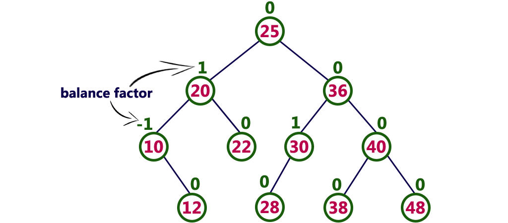
The above is an example of an AVL Tree with the balance factor of each node denoted above it.
Time and space complexity of AVL Tree operations
The Space complexity of AVL Tree is O(n) in average and worst case as we do not require any extra space to store duplicate data structures. The 'n' denotes the total number of nodes in the AVL tree. We come to this conclusion as each node has exactly 3 pointers i.e. left child, right child and parent. Each node takes up a space of O(1). And hence if we have 'n' total nodes in the tree, we get the space complexity to be n times O(1) which is O(n).
The various operations performed on an AVL Tree are Searching, Insertion and Deletion. All these are executed in the same way as in a binary search tree. The insert and delete operations may violate the property of AVL tree, hence checking the balance factor of every node after these operations is important.
Rotations in an AVL Tree
In case, any node of the tree becomes unbalanced, the required rotations are performed to restore the balance of the tree. There are four types of rotations possible. They are:
- LL Rotation: When the new node is inserted as the left child of the left subtree of the node which is imbalanced.
- RR Rotation: When the new node is inserted as the right child of the right subtree of the node which is imbalanced.
- LR Rotation: When the new node is inserted as the left child of the right subtree of the node which is imbalanced.
- RL Rotation: When the new node is inserted as the right child of the left subtree of the node which is imbalanced.
The first two types of rotations are single rotations and last two are double rotations.
In the best case scenario, rotations have a time complexity of O(1).
Derivation of height of an AVL tree
We know that for a binary search tree, the best height we can achieve is O(log n). Since AVL tree is also a variation of BST, its height in the best case also remaons the same. In the worst case, the height of BST is twice as deep as its optimal height. But in AVL tree, it still remains the same. Let us see the proof below.
Let us assume the height of the AVL tree to be h and the minimum number of nodes in the tree will be Nh. The height of the root would be 1 and one of its immediate child's subtree would have a height of h-1 and have Nh-1 nodes. Say that this is the right subtree. In the worst case, the balance factor of the root will be -1. So the subtree of left child of the root has a height of h-2 and has Nh-2 nodes. We now have a recurrence relation of form (Nh = Nh-1 + Nh-2 + 1).
Now we define the base cases. An AVL Tree with height 0 will have one node (just the root). Similarly, an AVL tree with height 1 will have a minimum of 2 nodes.
h = 0                   h = 1

  A            A                B
                \       or     /
                 B            A
Now that we have a recurrence relation and two base cases, we can reduce them as :
Nh = Nh-1 + Nh-2 + 1
Nh = ( Nh-2 + Nh-3 + 1) + Nh-2 + 1 ( as (Nh-1 = Nh-2 + Nh-3 + 1) from the recurrence relation)
Nh > 2 Nh-2
Nh > 2h/2
log (Nh) > log (2h/2)
2 log (Nh) > h
h = O (log (Nh))
Thus the height of an AVL tree in both best and worst case is O(log n).
Insertion
Inserting an element into an AVL tree requires rotations, calculating the balance factor and updating the height after insertion. As stated above, rotations are constant time operations. Calculating the balance factor and updating the height also takes up constant time. So the time consuming operation is traversing the length of the tree whose height is O(log n) .
-
The best case scenario is when no rebalancing is required and we can insert the new node in its position without making any structural changes to the tree. Here the time complexity will be O(log n) as we traverse the height of the AVL Tree.
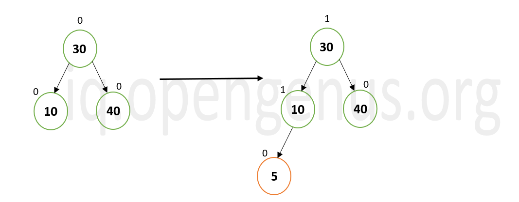
In the above example, when node 5 is inserted into the given tree, no changes are to be made to the tree as its balance is not disturbed. -
The worst case scenario is when after insertion of the new node, the tree becomes unbalanced and rotations are needed to be performed. Here too the time consumed is due to traversal which makes the time complexity as O(log n).
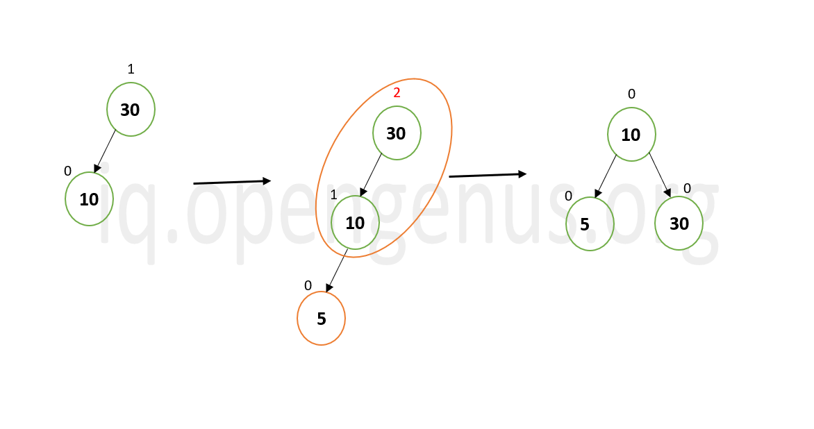
When we insert node 5 to the given tree, the balance factor of the root becomes 2 which violates the AVL Tree property. Thus we perform LL rotation to restore the tree's balance. -
Since the average case is the mean of all possible cases, the time complexity of insertion in this case too is O(log n).
Deletion
Similar to insertion, deletion too requires traversing the tree, calculating balance factor and updating the height of the tree after deletion of a particular node.
-
The best case scenario is when no rebalancing is required and deleting a node from the tree does not affect its balance. Here the time complexity will be O(log n) as we traverese the height of the AVL Tree to reach the node that is to be deleted.
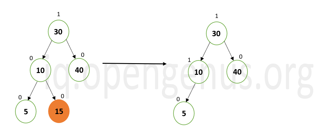
When the node 15 is deleted from the above given tree, no rotations are needed to be done as the tree still satisfies the AVL property. -
The worst case scenario is when after deletion of a particular node, the tree becomes unbalanced and rotations are needed to be performed. Here too the time consumed is due to traversal which makes the time complexity as O(log n).
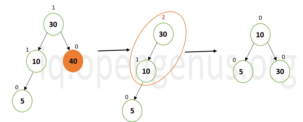
In the above given tree, when node 40 is deleted, the balance of the tree is disturbed as the balance factor of the root node becomes 2. Hence LL rotation is needed to be performed to restore the balance of the tree. -
Since the average case is the mean of all possible cases, the time complexity of deletion in this case too is O(log n).
Searching and Traversal
Traversal is an integral operation in AVL Tree which is used both in insertion and deletion. In all the three cases ( best case, wort case and average case), the traversal operation has a time complexity of O(log n).
As for searching an element in the AVL Tree, the time complexity in various cases is as follows:
- The best case scenario is when the element to be found is the root element itself. Hence, the element is found in the first pass and traversing the whole tree is not necessary. This makes the time complexity as O(1).
- The worst case is when the element to be found is present in one of the leaf nodes of the tree and we have to traverse throughout the length of the tree to find it. Hence the time complexity will be O(log n).
- The average case time complexity for searching is also O(log n).
Conclusion
To summarize , all the time complexities and space complexity have been listed in a tabluar form below.
Time Complexity:
| Operation | Best case | Average case | Worst case |
|---|---|---|---|
| Insert | O (log n) | O (log n) | O (log n) |
| Delete | O (log n) | O (log n) | O (log n) |
| Search | O (1) | O (log n) | O (log n) |
| Traversal | O (log n) | O (log n) | O (log n) |
Space Complexity:
| Best case | Average case | Worst case |
|---|---|---|
| O (n) | O (n) | O (n) |
With this article at OpenGenus, you must have the complete idea of Time & Space Complexity of AVL Tree operations.