
Open-Source Internship opportunity by OpenGenus for programmers. Apply now.
In this article, we will understand the cross entropy method that is widely used as an optimization technique in machine learning.
Table of contents
- What is entropy?
- The cross entropy method
- Applications
What is entropy?
Before we get to know about cross entropy method, first we need to understand what is entropy. Entropy is defined as the level of 'surprise' in the variable's possible outcome.
Let us now talk about entropy and surprise in detail. Say we have a bag of 12 balls out of which 11 are white and 1 is black. When we randomly pick a ball from this bag, we won't be much surprised if it turns out to be a white ball, since we already know that the majority of the balls in the bag are white. On the other hand, if the ball we picked turns out to be a black ball, we will be much more surprised. From this example, we can decipher that surprise is inversely related to probability.
Surprise is calculated as the log of the inverse of the probability. Its formula is:
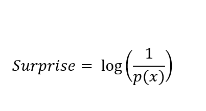
where p(x) is the probability of the event x happening.
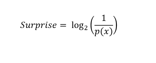
When we are calculating surprise for two outputs ( here, the two outputs are black ball and white ball), we usually use log base 2. The equation in this case becomes,
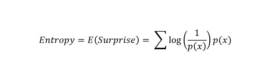
Now, Entropy is the expected value of surprise. To find the entropy for an event, we simply add the probability of the event with its surprise. Its formula is as follows:
Applying the properties of logarithms to the above equation and simplifying it, we get the equation of entropy that is widely used.
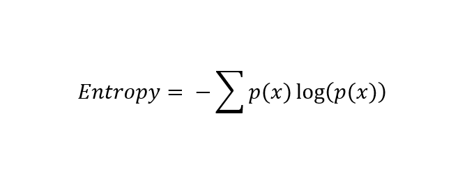
Entropy is also widely defined as the number of bits used to transmit an event, that is randomly selected from a probability distribution.
The cross entropy method
In machine learning, cross entropy is commonly used as a cost function when we are training classifiers.
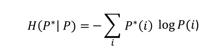
Cross entropy gives us an idea of how different two probability distributions for a given set of events are.
It is the summation of the true probability multiplied by the log predicted probability over all classes in the distribution. The formula for cross entropy is as follows:
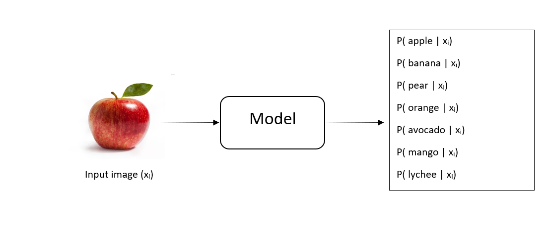
As an example, let us assume that we have the image of a fruit and we want the machine learning model to predict which class the image belongs to from a fixed set of possible fruit classes. A good model recognizes which class is most likely and it also recognizes the certainty we have of our prediction.
Now, when we give the image as an input to our model, it generates a probability distribution over the different fruit classes. Suppose we give an apple's image as an input. If our model is certain of its prediction, it assigns a probability of 1 to the class 'apple' and a probability of 0 to other fruit classes.
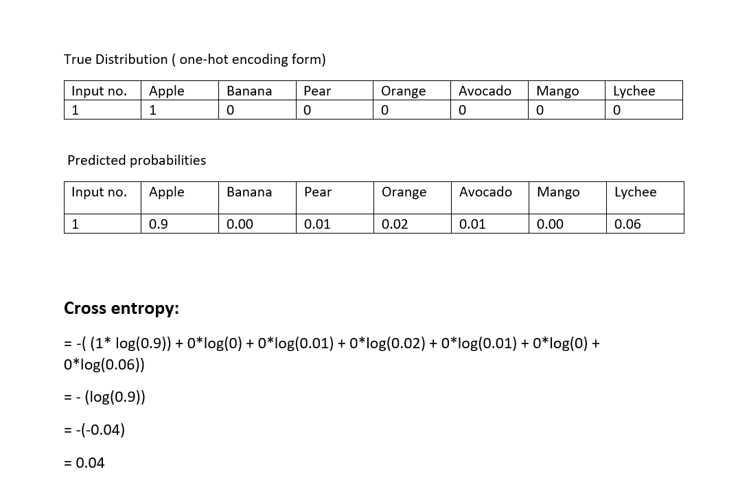
Now, suppose we know the true classes of out input images. This will be the true distribution (P*(x)) class and is also a vector. This vector will be in the one-hot encoding form.
To calculate the cross entropy of one event, we multiply the value in its corresponding one-hot encoding form with its predicted probability and get its product. We sum up all such products over different fruit classes.
Note that it is important to have softmax unit at the end of our model for it to generate valid probability distributions.
To get the total error for our model, all we need to do is to add up the cross entropy values of different inputs given. Based on the value we get, we can either use back propagation or adjust the weights to hopefully minimize the total error. This helps in minimizing the KL divergence and hence make models more accurate.
Cross entropy for optimization
The cross entropy method casts the original optimization problem into an estimation problem of rare-event probabilities. By doing so, this method aims to locate a probability distribution on the given set (Y) rather than directly finding the optimal solution.
Now, let us see the steps followed while using the cross entropy method for optimization.
Let us suppose that our goal is to find the maximum of a real-valued function S(x) over a given set Y where all x∈Y. Let γ be a threshold or level parameter and the random variable X has probability density function f(·; u), which is parameterized by a finite-dimensional real vector u( X ∼ f(·; u)). For simplicity, let us assume that there is only one maximizer x* . Let the maximum be denoted by γ* such that:
S(x* ) = γ* = max x∈YS(x) .
Let θ be the user defined parameter.
Given the sample size N and the parameter θ, execute the following steps:
- Choose an initial parameter vector v0. Let Ne = [θN]. Set level counter as t=1.
- Generate X1, . . . , XN ∼iid f(·; vbt−1). Calculate the performances S(Xi) for all i, and order them from smallest to largest: S(1) ≤ . . . ≤ S(N). Let γt be the sample (1−θ)-quantile of performances; that is, γt = S(N−Ne+1).
- Use the same sample X1, . . . , XN and solve the stochastic program
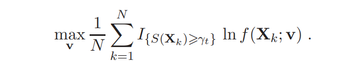
Denote the solution by vt. - If some stopping criterion is met, stop; otherwise, set t = t+1, and return to Step 2.
Applications
Knapsack packing problem
The Knapsack Problem is a constrained combinatorial optimization problem that refers to the general problem of packing a knapsack with the most valuable items without exceeding its weight limit. The best known variant of the KP is the 0-1 Knapsack Problem, which means that each item may be used or packed only once. It is defined as:
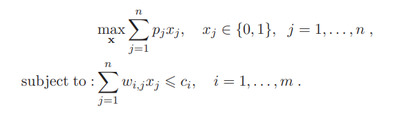
where, pj and wi,j are positive weights, ci is the positive cost parameter and x = (x1, . . . , xn). For getting a single objective function, we define:
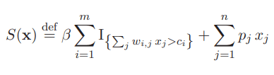
where β = −Σnj=1pj .
Let us consider the Sento1.dat knapsack problem. It contains 30 constraints and 60 variables. Since the solution vector x is binary, we choose the Bernoulli density as the sampling density. We apply the cross entropy method algorithm to this problem with the N=103, Ne=20 and v0 = (1/2 , ...... , 1/2). The solution for vt is given by:
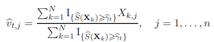
where Xk,j is the j-th component of the k-th random binary vector X.
We stop the algorithm if
dt=max1≤j≤n{min{vt,j,1-vt,j}} ≤ 0.01.
Max-cut problem
Consider a weighted graph G with node set V = {1, . . . , n}.Partition the nodes of the graph into two subsets V1 and V2 such that the sum of the weights of the edges going from one subset to the other is maximised.
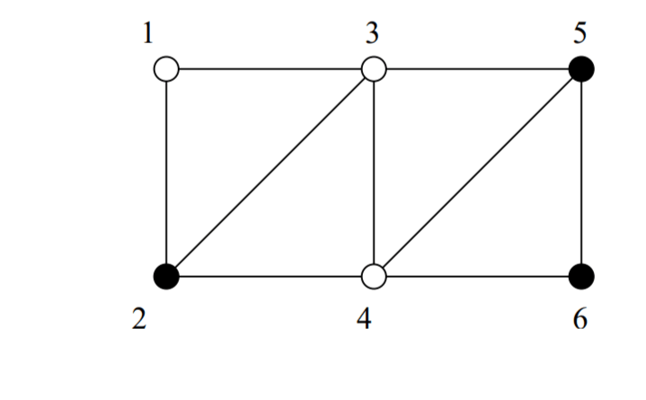
The cost matrix for the above graph will be:
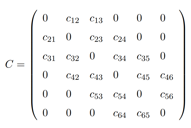
{V1, V2} = {{1, 3, 4}, {2, 5, 6}} is a possible cut. The cost of the cut is given by:
c12 + c32 + c35 + c42 + c45 + c46
We can represent a cut with the help of a cut vector x = (x1, . . . , xn), where xi = 1 if node i belongs to same partition as 1, and 0 if otherwise. For example, the cut {{1, 3, 4}, {2, 5, 6}} can be represented as (1, 0, 1, 1, 0, 0), which is a cut vector. Let X be the set of all cut vectors x = (1, x2, . . . , xn) and S(x) be the corresponding cost of the cut. Our aim is to maximize S(x).
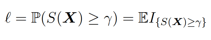
- First, cast the original optimization problem of S(x) into an associated rare-events estimation problem: the estimation of
- Second, formulate a parameterized random mechanism to generate objects X ∈ X . Then, iterate the following steps:
- Generate a random sample of objects X1, . . . , XN ∈ X (e.g.,cut vectors).
- Update the parameters of the random mechanism (obtained from CE minimization), in order to produce a better sample in the next iteration.
Here, the most natural and easiest way to generate the cut vectors is to let X2, . . . , XN be independent Bernoulli random variables with success probabilities p2, . . . , pn.
With this article at OpenGenus, you must have the complete idea of Cross entropy method for optimization.