In this article, we will explore various techniques used for optimizing hyperparameters of the machine learning model such as Grid Search, Bayesian Optimization, Halving randomized search and much more.

Table of contents

• Introduction
• Manual search
• Grid Search
• Randomized search
• Bayesian Optimization
• Halving grid search
• Halving randomized search
• Choosing the best model
  
  

Introduction

A machine learning model has two parameters: Hyperparameters and model parameters. Hyperparameters are the parameters whose values we arbitrarily set before training our model. They determine the structure of our model. Eg: learning rate for training a neural network. Model parameters are those whose values the model learns by itself while training. They tell the model how to use the input data to obtain the desired output. Eg: weights in neural network.

Hyperparameter optimization refers to tweaking the hyperparameters to get the right combination of them to either maximize or minimize a function. This is a lengthy process and has an impact on the performance of the model. There are several ways to optimize hyperparameters. They are:

• Grid search
• Randomized search
• Manual search
• Halving grid search
• Halving randomized search
• Automated Hyperparameter Tunings

In this article, we will discuss in detail about Manual, Grid and randomized search. To understand the concept behind these techniques, we will build a model to classify Iris flowers based on the attributes given. Let us consider support vector classifier (comes under SVM) as our model.

First, we import the dataset and svm from the sklearn library.

from sklearn import svm, datasets
iris = datasets.load_iris()

Then we convert the imported dataset into a dataframe.

import pandas as pd
df = pd.DataFrame(iris.data,columns=iris.feature_names)
df['flower'] = iris.target
df['flower'] = df['flower'].apply(lambda x: iris.target_names[x])
df.sample(6)

Our dataframe now looks as follows.

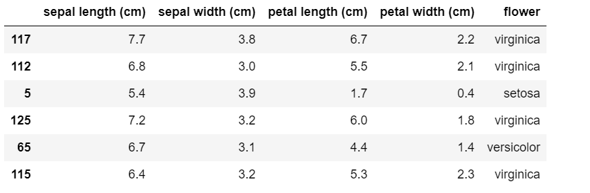
The three hyperparameters in SVM are 'C' , 'kernel' and 'gamma'. Now we will have a look at different techniques to tune these hyperparameters.

Manual search

Manual search is where we manually find the right combination of the hyperparameters and set them. This is a tedious process.

First, we try to find the right values by splitting the data using train_test_split and then plugging in the values of hyperparameters. This is a trial and error method. For each combination, we check the model score to see which is the best fit. For this, we import train_test_split and split the data. The code snippet is given below.

from sklearn.model_selection import train_test_split
X_train, X_test, y_train, y_test = train_test_split(iris.data, iris.target, test_size=0.3)

Now we manually tune parameters by trial and error.

model = svm.SVC(kernel='rbf',C=30,gamma='auto')
model.fit(X_train,y_train)
model.score(X_test, y_test)

Output:
0.9777777777777777

model = svm.SVC(kernel='rbf',C=20,gamma='scale')
model.fit(X_train,y_train)
model.score(X_test, y_test)

Output:
0.9777777777777777

model = svm.SVC(kernel='poly',C=10,gamma='auto')
model.fit(X_train,y_train)
model.score(X_test, y_test)

Output:
0.9777777777777777

model = svm.SVC(kernel='poly',C=20,gamma='scale')
model.fit(X_train,y_train)
model.score(X_test, y_test)

Output:
1.0

This process is unreliable as the scores change if we change the train and test sizes.

K-fold cross validation for manual search

For a more reliable manual search, we manually try suppling models with different parameters to cross_val_score function with K-fold cross validation. Here we chose our k-value to be 5. We first import cross_val_score.

from sklearn.model_selection import cross_val_score

Now we plug values into the cross_val_score function.

cross_val_score(svm.SVC(kernel='linear',C=10,gamma='auto'),iris.data, iris.target, cv=5)

Output:
array([1.        , 1.        , 0.9       , 0.96666667, 1.        ])

cross_val_score(svm.SVC(kernel='rbf',C=10,gamma='auto'),iris.data, iris.target, cv=5)

Output:
array([0.96666667, 1.        , 0.96666667, 0.96666667, 1.        ])

cross_val_score(svm.SVC(kernel='rbf',C=20,gamma='auto'),iris.data, iris.target, cv=5)

Output:
array([0.96666667, 1.        , 0.9       , 0.96666667, 1.        ])

This approach is very tiresome as it requires a lot of manual inputs. Instead, we can use loop as an alternative. For this, we import numpy package.

import numpy as np
kernels = ['rbf', 'linear']
C = [1,10,20]
gamma= ['scale','auto']
avg_scores = {}
for kval in kernels:
    for cval in C:
        for gval in gamma:
                    cv_scores = cross_val_score(svm.SVC(kernel=kval,C=cval,gamma=gval),iris.data, iris.target, cv=5)
                    avg_scores[kval + '_' + str(cval)] = np.average(cv_scores)

avg_scores

Now we get outputs for the different parameter values.

Output:
{'rbf_1': 0.9800000000000001,
 'rbf_10': 0.9800000000000001,
 'rbf_20': 0.9666666666666668,
 'linear_1': 0.9800000000000001,
 'linear_10': 0.9733333333333334,
 'linear_20': 0.9666666666666666}

From above results we can say that rbf with C=1 or 10 or linear with C=1 will give the best performance.

Grid Search

Grid search ca be described as a simpler and automated version of manual search. It does the same thing as our for loop implementation of manual search above, but in a single line of code. Here, we set up a grid of our parameters and then the model is trained/tested on each of the possible combinations. Computational time for grid search is very high as it tries out all the possible combinations of parameters in the grid. In python, we implement grid search using GridSearchCV.

from sklearn.model_selection import GridSearchCV

clf=GridSearchCV(svm.SVC(), {
    'C': [1,10,20,30],
    'kernel': ['rbf','linear','poly'],
    'gamma': ['scale','auto']
}, cv=5, return_train_score=False)
clf.fit(iris.data, iris.target)
df = pd.DataFrame(clf.cv_results_) #printing results as a dataframe
df

Our resulting dataframe looks as follows.

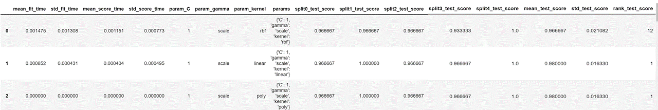
This displays the parameters used for each iteration, the test score for each split of cross validation and the mean of all the test scores. We now sort the values in descending order of column 'mean_test_score' and display the columns that we need.

df=df.sort_values(by='mean_test_score',ascending=False)
df[['param_C','param_kernel','param_gamma','mean_test_score']]

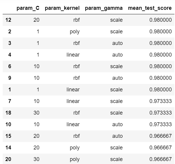
As we can see, we have several combinations that give us the maximum score of 0.98. To choose the best one, we just execute the following code.

clf.best_params_

Output:
{'C': 1, 'gamma': 'scale', 'kernel': 'linear'}

Now, we got the right combination of parameters for our model using grid search.

Randomized search

Randomized search is the same as grid search. The only difference is that instead of trying out all the combinations of parameters in the grid, it just tries out random combinations. This reduces the number of iterations and is useful when we have too many parameters to try. It helps reduce the cost of computation. Randomized search is implemented in python using RandomizedSearchCV.

from sklearn.model_selection import RandomizedSearchCV
rs = RandomizedSearchCV(svm.SVC(gamma='auto'), {
        'C': [1,10,20,30],
        'kernel': ['rbf','linear','poly'],
        'gamma': ['scale','auto']
    }, 
    cv=5, 
    return_train_score=False, 
    n_iter=3
)
rs.fit(iris.data, iris.target)
pd.DataFrame(rs.cv_results_)[['param_C','param_kernel','mean_test_score']]

Here, n_iter refers to the number of combinations to be tried out randomly. The output is given below.

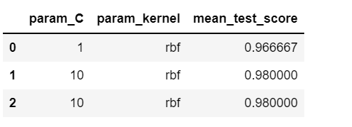
This changes every time we execute the code as different samples are chosen randomly every time.

Bayesian optimization

The goal of Bayesian optimization is to find an input value to a function that returns the lowest possible output and is an example of automated hyperparameter tuning. This uses probability to achieve the same. Bayesian Grid Search models the search space using Bayesian optimization. It uses candidates from previous evaluations to sample out the candidates that might give better results. In python, Bayesian optimization can be implemented using the hyperopt library. Hyperopt-sklearn is an extension of the hyperopt library. For implementing Bayesian Grid Search, we use scikit-optimize (skopt) library.

from skopt import BayesSearchCV
search_spaces = {"C": [1,10,20,30],
                 "kernel": ['rbf','linear','poly'],
                 "gamma": ['scale','auto']}
opt = BayesSearchCV(model, search_spaces, cv=5)
opt.fit(X_train, y_train)

Now we find the best score and best parameters.

opt.best_score_

Output:
0.9714285714285715

opt.best_params_

Output:
OrderedDict([('C', 1), ('gamma', 'auto'), ('kernel', 'rbf')])

Halving grid search

Halving grid search uses a technique known as successive halving. It trains all possible hyperparameter combinations on a small portion of training data, instead of the whole training data. In the next iteration, only the combination of parameters that gave good results are considered. This is continued until the only survivor is the best combination of parameters.

from sklearn.experimental import enable_halving_search_cv 
from sklearn.model_selection import HalvingGridSearchCV

halving_cv = HalvingGridSearchCV(model, {
    'C': [1,10,20,30],
    'kernel': ['rbf','linear','poly'],
    'gamma': ['scale','auto']
})
halving_cv.fit(X_train, y_train)

print("Best Params", halving_cv.best_params_)
print("Best CV Score", halving_cv.best_score_)

Best Params {'C': 1, 'gamma': 'auto', 'kernel': 'rbf'}
Best CV Score 0.9777777777777779

The results vary each time we execute the above code snippet as a different portion of training dataset is chosen each time.

Halving randomized search

Halving randomized search also uses the same successive halving approach. Unlike halving grid search, it trains just randomly selected combinations of parameters on a portion of the training data.

from sklearn.model_selection import HalvingRandomSearchCV

halving_rcv = HalvingRandomSearchCV(model, {
    'C': [1,10,20,30],
    'kernel': ['rbf','linear','poly'],
    'gamma': ['scale','auto']
})
halving_rcv.fit(X_train, y_train)

print("Best Params", halving_rcv.best_params_)
print("Best CV Score", halving_rcv.best_score_)

Output:
Best Params {'kernel': 'rbf', 'gamma': 'auto', 'C': 20}
Best CV Score 0.9555555555555555

The output of this too varies every time.

Choosing the best model

We found the best parameter values for SVM. But is that the best model for our dataset? To check that, we find the best values the hyperparameters for different machine learning models and compare them. Here, the models we will be testing out are Random forest, Logistic regression and SVM. We import the required libraries and then give the parameter values for different models as a dictionary.

from sklearn import svm
from sklearn.ensemble import RandomForestClassifier
from sklearn.linear_model import LogisticRegression

model_params = {
    'svm': {
        'model': svm.SVC(),
        'params' : {
            'C': [1,10,20,30],
            'kernel': ['rbf','linear','poly'],
            'gamma': ['scale','auto']
        }  
    },
    'random_forest': {
        'model': RandomForestClassifier(),
        'params' : {
            'n_estimators': [1,5,10,15]
        }
    },
    'logistic_regression' : {
        'model': LogisticRegression(solver='liblinear',multi_class='auto'),
        'params': {
            'C': [1,5,10,15]
        }
    }
}

Now, we perform grid search over the parameters of each model and get its best score to find the best fit model.

scores = []

for model_name, mp in model_params.items():
    clf =  GridSearchCV(mp['model'], mp['params'], cv=5, return_train_score=False)
    clf.fit(iris.data, iris.target)
    scores.append({
        'model': model_name,
        'best_score': clf.best_score_,
        'best_params': clf.best_params_
    })
    
df = pd.DataFrame(scores,columns=['model','best_score','best_params'])
df

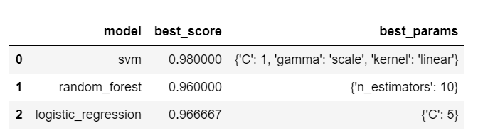
Based on above output, we can conclude that SVM with C=1 and kernel='rbf' is the best model for solving our problem of iris flower classification.

With this article at OpenGenus, you must have the complete idea of Different Hyperparameter optimization techniques.