
Get this book -> Problems on Array: For Interviews and Competitive Programming
Deep learning has many applications in versatile fields like: automobiles, home appliances and manufactoring. In this article we will build a fault detection system using a deep learning model : EfficientNet to distinguish between defective and non-defective cells that are extracted from solar modules.
You should follow this guide and prepare your own version. This Deep Learning Project is a strong addition to ML Engineer Portfolio.
Table of content
- Dataset Description
- Data Exploration
- Data pre-processing
- Building the model
- Evaluation using Grad-CAM
- Conclusion
1. Dataset Description
The dataset used in this article can be downloaded from here. It is composed of 2624 grayscale images of size 300x300. Each image represent a cell that was extracted from a solar module. But what is a solar module?
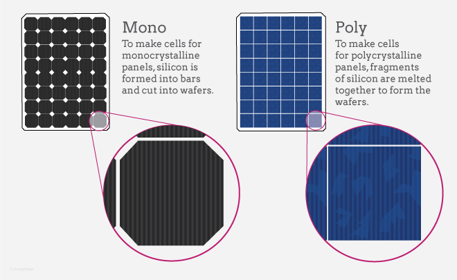
Solar Module is an assembly of solar cells that absorb sunlight as a source of energy to produce electricity. There are three types of solar modules: Mono-crystalline Solar Modules, Polycrystalline Solar Modules and Thin-film Solar Modules.
In this dataset, the cells were extracted from a mono-crystalline solar module and a polycrystalline one. For those who are curious like me, here is the difference between the two :
Mono-crystalline solar panels have solar cells made from a single crystal of silicon while polycrystalline solar panels have solar cells made from several fragments of silicon melted together.
Going back to our main topic, the images contain non-defective and defective cells. The annotations of the dataset can be found in the file labels.csv where each row has:
- The image path
- The probability of being defective
- The type of the solar module from which the cell was extracted.
2. Data Exploration
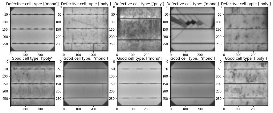
Let's start by visualizing some images from our dataset.
First we will be creating a function that will load the dataset and transforms the categorical features (the cell type) to numerical features. Also, since our target variable is a probability of being defective or not, we will apply to it a threshold of 50%. So if the probability is higher or equal to 0.5 then the target variable will be set to 1 elsewhere it will be set to 0.
# import required packages
import pandas as pd
import numpy as np
import matplotlib.pyplot as plt
from sklearn.model_selection import train_test_split
from utils.elpv_reader import load_dataset
import tensorflow as tf
from tensorflow.keras import layers
from tensorflow.keras.utils import to_categorical
def load_data():
  images, probas, labels = load_dataset()

  # Convert the type of the solar module
  # to numerical values
  labels[labels == "mono"] = 0
  labels[labels == "poly"] = 1

  # Convert the probabilities to classes
  probas[probas >= 0.5] = 1. # the cell is defective
  probas[probas < 0.5] = 0. # the cell is not defective

  # Convert grayscale to rgb
  # This is needed to adapt the data
  # to the model's input format
  rgb_imgs = np.repeat(images[..., np.newaxis],3,-1)

  # The images and the type of the cell
  # are going to be the inputs to our model
  X1 = rgb_imgs
  X2 = labels

  # The probabilities of being defective
  # are going to be the outputs of our model
  Y = probas

  return X1,X2,Y

X1,X2,Y = load_data()
defective_images = X1[Y == 1][:10]
non_defective_images = X1[Y == 0][:5]

cell_types_def = X2[Y== 1][:5]
cell_types_ndef = X2_train[Y == 0][:5]

plt.figure(figsize=(15,6))

for i in range(5):
    plt.subplot(2,5,i+1)
    plt.imshow(defective_images[i,...])
    plt.title(f"Defective cell type: {cell_types_def[i]}")

for i in range(5,10):
    plt.subplot(2,5,i+1)
    plt.imshow(non_defective_images[i-5,...])
    plt.title(f"Good cell type: "+ "Poly" if cell_types_ndef[i-5]== 1 else "Mono")
Next we will see the range of pixel intensities in the images
min_intensity = np.min(X1)
max_intensity = np.max(X1)

print(f"The range of pixel intensities is between {min_intensity}-{max_intensity}")

output:
The range of pixel intensities is between 0-255
Finally, we will verify whether our dataset is balanced or not
pos_class = np.sum(Y)/len(Y)*100
neg_class = (len(Y)-np.sum(Y))/len(Y)*100

print(f'The dataset has {np.round(pos_class,2)} % defective cells and {np.round(neg_class,2)} % non-defective cells')

output:
The dataset has 31.29 % defective cells and 68.71 % non-defective cells
Our dataset is clearly imbalanced. As a remedy to this we will be using a weighted loss to train our model.
3. Data preprocessing
For the moment, you may have noticed that we have two features we can input to our deep learning model: the images and the type of the cells.
So which one are we going to use? and is it possible to input both?
The answer is yes, we can input both features to the model. However, for the sake of simplicity, in this article, we will be using only the images as inputs.
Before preprocessing the images, we will split our dataset to training and validation sets, using the stratified strategy to make sure that both sets have the same proportion of classes.
Then we will be using the Tensorflow ImageDataGenerator class to pre-process and augment the images.
# Convert target variable to binary class matrix
Y = to_categorical(Y)

# Splitting the dataset
X1_train,X1_val,Y_train,Y_val = train_test_split(X1,Y,test_size=0.2,random_state=13,stratify=Y)

print(f"Training set size: {X1_train.shape} \nValidation set size: {X1_val.shape}")

output:
Training set size: (2099, 300, 300, 3)
Validation set size: (525, 300, 300, 3)
As a preprocessing step, we need to resize all the images (training and validation images) to (224,224) and also rescale the range of pixel intensities to the range 0-1 (This helps to stabilize the gradient descent step, allowing us to use larger learning rates or help models converge faster for a given learning rate).
As a Data-augmentation strategy, we will use: random_shear, random zoom, random translation and then random horizontal and vertical flip. But, it is going to be implemented only on the training dataset.
BATCH_SIZE = 32
# this is the default size used by most of the pretrained Keras models
image_size = (224, 224)

train_datagen = tf.keras.preprocessing.image.ImageDataGenerator(
        samplewise_center=False,
        samplewise_std_normalization=False,
        rescale=1./255,
        shear_range=0.2, # do some data augmentation here
        zoom_range=0.2,
        rotation_range=30,
        horizontal_flip=True,
        vertical_flip=True)

# create testing and validation data generator without augmentation
val_datagen = tf.keras.preprocessing.image.ImageDataGenerator(
        samplewise_center=False,
        samplewise_std_normalization=False,
        rescale=1./255
        )


train_ds = train_datagen.flow(x=tf.image.resize(X1_train,size=image_size),
                              y=Y_train,
                              batch_size=BATCH_SIZE)#, class_mode='binary')
val_ds = val_datagen.flow(x=tf.image.resize(X1_val,size=image_size),
                          y=Y_val,
                          batch_size=BATCH_SIZE)
4. Building the model
As mentioned before the dataset is too small and can't be used to train a robust model from scratch, hence we will be using a strategy called Transfer Learning. So what is Transfer Learning?
Transfer Learning is a machine learning method where we take a pre-trained model on some auxilary task and use it as a starting point for another model that we wish to train on a desired task. This technique helps faster progress when modeling for the second task.
In our case, we will be using EfficientNetV2B2 that is trained on ImageNet dataset. EfficientNetV2B2 is one of the less complex versions of EfficientNetV2 models. The reason behind choosing this verison not others is because higher version (>=B3) are large and complex models thus using one of them as a base model for our small dataset will only cause the new model to overfit (you can try it for yourself and verify :) ).
With that beign said, Let's jump to the coding part.
First, we need to choose which layers from EfficientNetV2B2 we are going to use for feature extraction. If you are familiar with CNNs, you may know that the features are stored in the filter maps. Thus, the very last classification layer is not much useful in our case, instead we need the feature maps that are just before the last Flatten layer. To do so, we need to specify include_top = False when calling the model.
base_model = tf.keras.applications.EfficientNetV2B2(input_shape=input_shape,
                                                     input_tensor=inputs,
                                                     include_top=False,
                                                     weights='imagenet',
                                                  include_preprocessing=False,
                                                   )
Next, we need to specify that the weights of the base_model should not be updated by executing the following instruction:
# Freezing all convoltional layers
# in the base_model
base_model.trainable = False
Finally, let's create a function that will create the new model.
def create_transfer_learning_model(
                                   fine_tune=False,
                                   fine_tune_at=None,
                                   input_shape=(224,224,3),
                                   base_learning_rate = 0.00001
                                   ):


    inputs = tf.keras.Input(shape=input_shape)
    base_model = tf.keras.applications.EfficientNetV2B2(input_shape=input_shape,
                                                     include_top=False,
                                                     input_tensor=inputs,
                                                     weights='imagenet',
                                                     include_preprocessing=False,
                                                   )
    # Freeze the base model
    base_model.trainable = False

    if fine_tune :
        if not fine_tune_at:
            raise Exception("You should specify from which"+
                            " layer the model will be fine tuned"
                            )
        else:
            base_model.trainable = True

            # Freeze the lowest layers
            # and fine tune the top layers
            # starting from index "fine_tune_at"
            for layer in base_model.layers[:fine_tune_at]:
                layer.trainable = False

    x = base_model.output
    x = layers.BatchNormalization()(x)
    x = layers.GlobalAveragePooling2D()(x)
    x = layers.BatchNormalization()(x)
    x = tf.keras.layers.Dropout(0.2)(x)

    outputs = layers.Dense(2,activation="softmax")(x)

    model = tf.keras.Model(inputs, outputs)

    # Compile the model
    model.compile(optimizer=tf.keras.optimizers.Adam(learning_rate=base_learning_rate),
                  loss= tf.keras.losses.CategoricalCrossentropy(from_logits=False),
                  metrics=[tf.keras.metrics.CategoricalAccuracy()])
    return model, base_model

model, base_model = create_transfer_learning_model()
model.summary()
output:
Model: "model"
__________________________________________________________________________________________________
 Layer (type)                   Output Shape         Param #     Connected to
==================================================================================================
 input_1 (InputLayer)           [(None, 224, 224, 3  0           []
                                )]
 stem_conv (Conv2D)             (None, 112, 112, 32  864         ['input_1[0][0]']
                                )
 stem_bn (BatchNormalization)   (None, 112, 112, 32  128         ['stem_conv[0][0]']
                                )
 stem_activation (Activation)   (None, 112, 112, 32  0           ['stem_bn[0][0]']
                                )
 block1a_project_conv (Conv2D)  (None, 112, 112, 16  4608        ['stem_activation[0][0]']

 ......

top_conv (Conv2D)              (None, 7, 7, 1408)   292864      ['block6j_add[0][0]']

 top_bn (BatchNormalization)    (None, 7, 7, 1408)   5632        ['top_conv[0][0]']
 top_activation (Activation)    (None, 7, 7, 1408)   0           ['top_bn[0][0]']
 batch_normalization (BatchNorm  (None, 7, 7, 1408)  5632        ['top_activation[0][0]']
 alization)
 global_average_pooling2d (Glob  (None, 1408)        0           ['batch_normalization[0][0]']
 alAveragePooling2D)
 batch_normalization_1 (BatchNo  (None, 1408)        5632        ['global_average_pooling2d[0][0]'
 rmalization)                                                    ]
 dropout (Dropout)              (None, 1408)         0           ['batch_normalization_1[0][0]']
 dense (Dense)                  (None, 2)            2818        ['dropout[0][0]']
==================================================================================================
Total params: 8,783,456
Trainable params: 8,450
Non-trainable params: 8,775,006
Since, our dataset is imbalanced we need to pass the weights of the classes to the loss function to prevent the model from being biased toward a particular class.
To compute the weights for each class we can use scikit-learn function class_weight like follow
from sklearn.utils import class_weight

# Calculate the weights for each class so that we can balance the data
weights = class_weight.compute_class_weight(class_weight = "balanced",
                                        classes = np.unique(Y_train),
                                        y = Y_train)
# weights should be a dictionary
#
weights = dict(zip(np.unique(Y_train), weights))
We also need to define some callbacks: one to save the best model, one to decrease the learning rate and finally one to save the steps of the training
score.
# Define Callbacks to save the best model
if not os.path.exists("./models/"):
  os.makedirs("./models/")

chkp_filepath= "./models/best_efficient_net_b2_final2_{epoch:02d}.h5"
checkpoint = tf.keras.callbacks.ModelCheckpoint(chkp_filepath, verbose=1,
                             save_best_only=True,monitor="val_categorical_accuracy",mode='max',save_freq="epoch")

# Callback to save the training history
filename='logs_effecient_net_b2_final.csv'
history_logger= tf.keras.callbacks.CSVLogger(filename, separator=",", append=True)

'Custom callback to decrease learning rate by a factor of 3 every 2 epoch'
class DecreaseLR(tf.keras.callbacks.Callback):
    def on_epoch_end(self, epoch, logs=None):
        if epoch > 4 and epoch % 2 == 0:
            self.model.optimizer.lr = self.model.optimizer.lr / 3
Finally, we fit the model for 18 epochs
from sklearn.utils import class_weight

# Calculate the weights for each class so that we can balance the data
# y = np.argmax(Y_train,axis=-1)
# weights = class_weight.compute_class_weight(class_weight = "balanced",
#                                        classes = np.unique(y),
#                                        y = y)
# weights = dict(zip(np.unique(Y_train), weights))
weights = {0.0:0.5, 1.0:1.5}

initial_epochs = 18
history = model.fit(train_ds,
                    epochs=initial_epochs,
                    validation_data=val_ds,
                    callbacks=[history_logger, checkpoint,DecreaseLR()],
                    class_weight=weights
                    )
Output:
Epoch 1/18
66/66 [==============================] - ETA: 0s - loss: 1.0448 - categorical_accuracy: 0.6465
Epoch 1: val_categorical_accuracy improved from -inf to 0.79810, saving model to ./models/best_efficient_net_b2_final2_01.h5
66/66 [==============================] - 37s 424ms/step - loss: 1.0448 - categorical_accuracy: 0.6465 - val_loss: 0.4521 - val_categorical_accuracy: 0.7981
Epoch 2/18
66/66 [==============================] - ETA: 0s - loss: 1.1372 - categorical_accuracy: 0.6698
Epoch 2: val_categorical_accuracy did not improve from 0.79810
66/66 [==============================] - 24s 359ms/step - loss: 1.1372 - categorical_accuracy: 0.6698 - val_loss: 0.5116 - val_categorical_accuracy: 0.7257
Epoch 3/18
66/66 [==============================] - ETA: 0s - loss: 0.9360 - categorical_accuracy: 0.6960
Epoch 3: val_categorical_accuracy did not improve from 0.79810
66/66 [==============================] - 24s 361ms/step - loss: 0.9360 - categorical_accuracy: 0.6960 - val_loss: 1.1826 - val_categorical_accuracy: 0.6248
Epoch 4/18
66/66 [==============================] - ETA: 0s - loss: 0.9189 - categorical_accuracy: 0.6803
Epoch 4: val_categorical_accuracy did not improve from 0.79810
66/66 [==============================] - 24s 360ms/step - loss: 0.9189 - categorical_accuracy: 0.6803 - val_loss: 0.5224 - val_categorical_accuracy: 0.7790
Epoch 5/18
66/66 [==============================] - ETA: 0s - loss: 0.9548 - categorical_accuracy: 0.6684
Epoch 5: val_categorical_accuracy did not improve from 0.79810
66/66 [==============================] - 25s 384ms/step - loss: 0.9548 - categorical_accuracy: 0.6684 - val_loss: 0.7560 - val_categorical_accuracy: 0.7219
Epoch 6/18
66/66 [==============================] - ETA: 0s - loss: 0.8936 - categorical_accuracy: 0.6760
Epoch 6: val_categorical_accuracy did not improve from 0.79810
66/66 [==============================] - 24s 363ms/step - loss: 0.8936 - categorical_accuracy: 0.6760 - val_loss: 0.8658 - val_categorical_accuracy: 0.7962
Epoch 7/18
66/66 [==============================] - ETA: 0s - loss: 0.7965 - categorical_accuracy: 0.6832
Epoch 7: val_categorical_accuracy improved from 0.79810 to 0.82857, saving model to ./models/best_efficient_net_b2_final2_07.h5
66/66 [==============================] - 27s 415ms/step - loss: 0.7965 - categorical_accuracy: 0.6832 - val_loss: 0.4835 - val_categorical_accuracy: 0.8286

...

Epoch 12/18
66/66 [==============================] - ETA: 0s - loss: 0.4999 - categorical_accuracy: 0.7132
Epoch 12: val_categorical_accuracy improved from 0.82857 to 0.83619, saving model to ./models/best_efficient_net_b2_final2_12.h5
66/66 [==============================] - 25s 377ms/step - loss: 0.4999 - categorical_accuracy: 0.7132 - val_loss: 0.4074 - val_categorical_accuracy: 0.8362
Epoch 13/18
66/66 [==============================] - ETA: 0s - loss: 0.4792 - categorical_accuracy: 0.7075
Epoch 13: val_categorical_accuracy did not improve from 0.83619
66/66 [==============================] - 24s 366ms/step - loss: 0.4792 - categorical_accuracy: 0.7075 - val_loss: 0.4315 - val_categorical_accuracy: 0.8152

...

Epoch 17/18
66/66 [==============================] - ETA: 0s - loss: 0.4630 - categorical_accuracy: 0.7208
Epoch 17: val_categorical_accuracy did not improve from 0.83619
66/66 [==============================] - 24s 364ms/step - loss: 0.4630 - categorical_accuracy: 0.7208 - val_loss: 0.4115 - val_categorical_accuracy: 0.8229
Epoch 18/18
66/66 [==============================] - ETA: 0s - loss: 0.4580 - categorical_accuracy: 0.7251
Epoch 18: val_categorical_accuracy did not improve from 0.83619
66/66 [==============================] - 26s 388ms/step - loss: 0.4580 - categorical_accuracy: 0.7251 - val_loss: 0.4117 - val_categorical_accuracy: 0.8210
Finally, let's visualize the evolution of the loss and accuracy
acc = history.history['categorical_accuracy']
val_acc = history.history['val_categorical_accuracy']

loss = history.history['loss']
val_loss = history.history['val_loss']

plt.figure(figsize=(8, 8))
plt.subplot(2, 1, 1)
plt.plot(acc, label='Training Accuracy')
plt.plot(val_acc, label='Validation Accuracy')
plt.legend(loc='lower right')
plt.ylabel('Accuracy')
plt.ylim([min(plt.ylim()),1])
plt.title('Training and Validation Accuracy')

plt.subplot(2, 1, 2)
plt.plot(loss, label='Training Loss')
plt.plot(val_loss, label='Validation Loss')
plt.legend(loc='upper right')
plt.ylabel('Cross Entropy')
plt.ylim([0,1.0])
plt.title('Training and Validation Loss')
plt.xlabel('epoch')
plt.show()
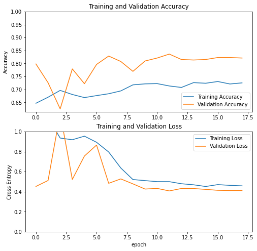
As we can see, both loss and accuracy are improving through time which means that our model was effectively learning. Also, we notice that the validation loss is better than the training loss and the validation accuracy is better than the training accuracy which proves that the model is generalizing well on new cases thus we have no overfitting problem.
5. Evaluation using Grad-CAM
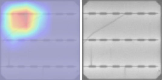
In this section, we will try to understand how the model is detecting the defective cells in our dataset using an algorithm called Grad-CAM.
Grad-CAM is a technique that uses the gradients of the classification scores with respect to the final convolutional feature map to create heat-maps that highlight the parts of an input image that most impact the classification score.
In our case, we will be using a variant of this algorithm called ScoreCam[5].
First, we need to install the package : tf-keras-vis
!pip install tf-keras-vis
Next we need to create a score function that will be passed to the ScoreCam algorithm. We have to options to achieve that :
- Either use the Tensorflow class CategoricalScore like follow :
from tf_keras_vis.utils.scores import CategoricalScore
score_function = CategoricalScore(labels.astype('int8').tolist())
- Or Define a costume method :
def score_function(output):
    # The `output` variable refers to the output of the model,
    # so, in this case, `output` shape is  (samples, nb_classes).
    return [output[i, labels[i].astype('int8')] for i in range(output.shape[0])]
Next you can call the ScoreCam Algorithm to generate the heatmaps of the predictions. We need to specify the last convolutional layer in the parameter penultimate_layer or let the algorithm find it by specifying seek_penultimate_conv_layer=True :
from tf_keras_vis.scorecam import Scorecam
# Create ScoreCAM object
scorecam = Scorecam(best_model)

# Generate heatmap with ScoreCAM
# images.shape = (batch_size,224,224,3)
cam = scorecam(score_function, images[9:10,...],
               penultimate_layer=-6,
               seek_penultimate_conv_layer= False)
Finally here is the result we got on a defective cell :
6. Conclusion
As a wrap up, in this article we saw an application of deep learning networks on a real world project: detecting defective solar module cells.
We learned about transfer learning technique and how it is useful when we have a small dataset.
We also learned about ScoreCam and used it to explain what the model is looking at while predicting the inputs.
You can challenge yourself and try to build a model with two inputs (using the type of the cell as a second feature). Also you can try and fine tune the base_model to see whether the accuracy improves, just make sure when doing so that your learning rate is really small to avoid making big changes on the weights.
Finally, you can find the full code of this project in the following github repo
References
[1] Buerhop-Lutz, C.; Deitsch, S.; Maier, A.; Gallwitz, F.; Berger, S.; Doll, B.; Hauch, J.; Camus, C. & Brabec, C. J. A Benchmark for Visual Identification of Defective Solar Cells in Electroluminescence Imagery. European PV Solar Energy Conference and Exhibition (EU PVSEC), 2018. DOI: 10.4229/35thEUPVSEC20182018-5CV.3.15
[2] Deitsch, S., Buerhop-Lutz, C., Sovetkin, E., Steland, A., Maier, A., Gallwitz, F., & Riess, C. (2021). Segmentation of photovoltaic module cells in uncalibrated electroluminescence images. Machine Vision and Applications, 32(4). DOI: 10.1007/s00138-021-01191-9
[3] Deitsch, S.; Christlein, V.; Berger, S.; Buerhop-Lutz, C.; Maier, A.; Gallwitz, F. & Riess, C. Automatic classification of defective photovoltaic module cells in electroluminescence images. Solar Energy, Elsevier BV, 2019, 185, 455-468. DOI: 10.1016/j.solener.2019.02.067
[4] Monocrystalline vs Polycrystalline Solar Panels. American Solar Energy Society [online]. 20 February 2021. Available from: https://ases.org/monocrystalline-vs-polycrystalline-solar-panels/
[5] WANG, Haofan, WANG, Zifan, DU, Mengnan, et al. Score-CAM: Score-weighted visual explanations for convolutional neural networks. In : Proceedings of the IEEE/CVF conference on computer vision and pattern recognition workshops. 2020. p. 24-25.