In this article, we will explore the various Monte Carlo sampling techniques used in Probability and Data Science.

Table of contents

• What are Monte Carlo techniques?
• Different Monte Carlo techniques for sampling
  * Importance Sampling
  * Rejection Sampling
  * Markov chain Monte Carlo (MCMC) sampling
  
  

What are Monte Carlo techniques?

Monte Carlo techniques are a group of computational algorithms for sampling probability distributions in a random manner. These were first used to solve the complicated diffusion problems in physics around the time when the first atomic bomb was being developed.

When we are predicting the probability or outcome of a bigger event that depends on a number of smaller events whose probabilities are difficult to predict due to random variables, we use Monte Carlo simulation to model the probabilities of different outcomes. For example, it can be used to calculate risks in business and the performance of stock market.

These methods can be used to solve:

• Problems that are stochastic in nature:
  * Particle transport
  * Population studies
• Problems that are deterministic in nature:
  * Solving partial differential equations and system of algebraic equations.
  * Evaluating integrals.

Steps to conduct a Monte Carlo simulation:

1. List all the possible outcomes.
2. Assign probabilities to each outcome.
3. Set up a correspondence between random numbers and each outcome.
4. Select random numbers and conduct the simulation.
5. Run the simulation as many times as required.
6. Compute the statistics.

Let us get an idea of this in mathematical terms. Suppose we need to evaluate ∫ p(x) f(x) dx where, x is a random variable that is continuous, p(x) is its probability density and f(x) is a scalar function of x that we are interested in. Many a times, it is impossible to calculate this integral exactly as the dimension of x is high. Here's where Monte Carlo methods help us. The basic idea of this method is to approximate the expectation of the value of the integral with an average as follows:

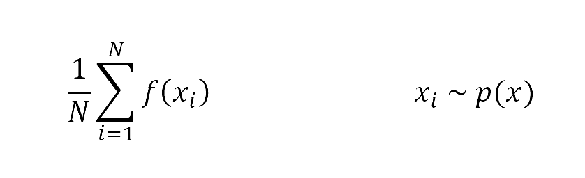
Here, we take N samples from p(x), put it into the function f(x) and take its average.

Different Monte Carlo techniques for sampling

There are different Monte Carlo methods based on the way the samples are chosen or the constraints on the sampling process. Here, we will have a look at two of those types:

• Importance Sampling
• Rejection Sampling
• Markov chain Monte Carlo (MCMC) sampling

Importance Sampling

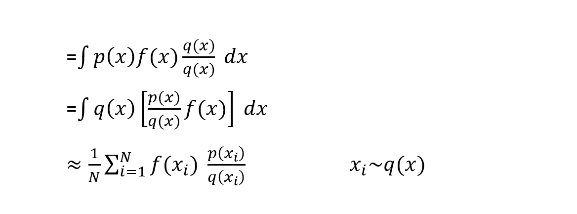
Consider the integral mentioned above. If p(x) is hard to sample from, we use importance sampling. Here, we sample from a simpler approximation of the target distribution (say q(x)).

The trick here is to multiply the equation with q(x)/q(x). Here, q(x)≠0 and p(x)f(x)≠0. The transformation looks as follows.

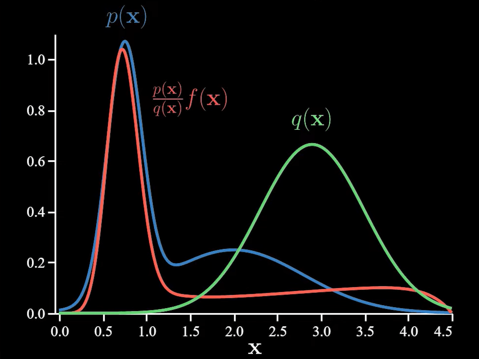
Let us take a look at an example. Let the functions p(x) and f(x) be as follows.

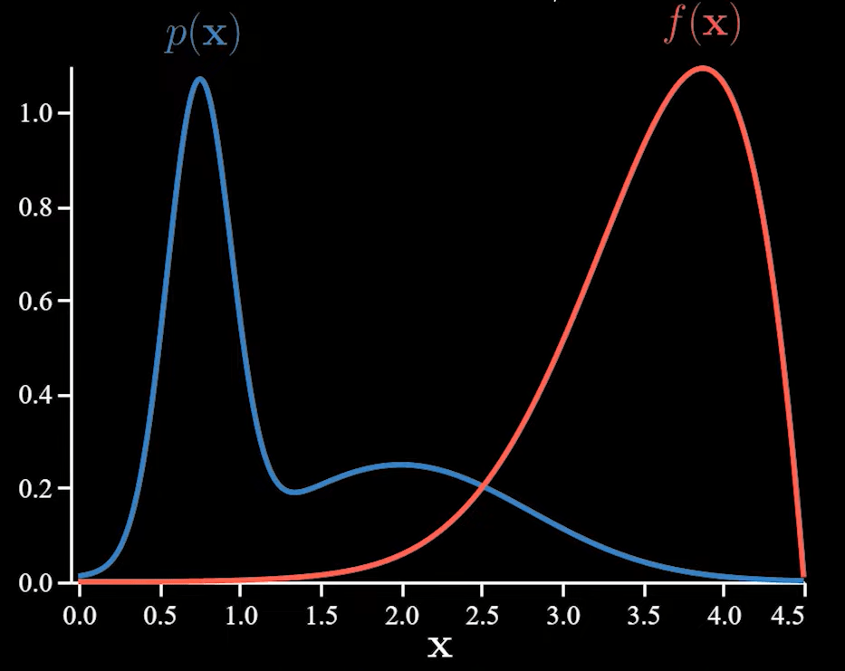
When we find the estimate without using importance sampling, we find that it varies a lot as the function f has large values only under a few events of p and these set of samples have an impact on the average.

Using importance sampling, we can sample the more important regions frequently. We take a distribution q(x).

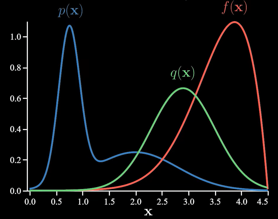
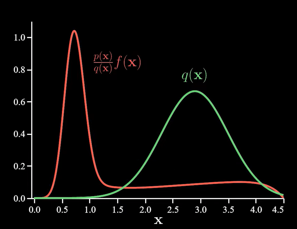
Since we are now sampling from q(x), we need to make adjustments to the function f(x) as discussed earlier.

Now, we eliminate p(x) and perform normal Monte Carlo sampling with the remaining functions.

Importance sampling is mainly used to reduce the variance.

Rejection Sampling

This sampling technique is used when our distribution is difficult to sample from. Here, we make use of a distribution that is easy to sample from as a proxy.

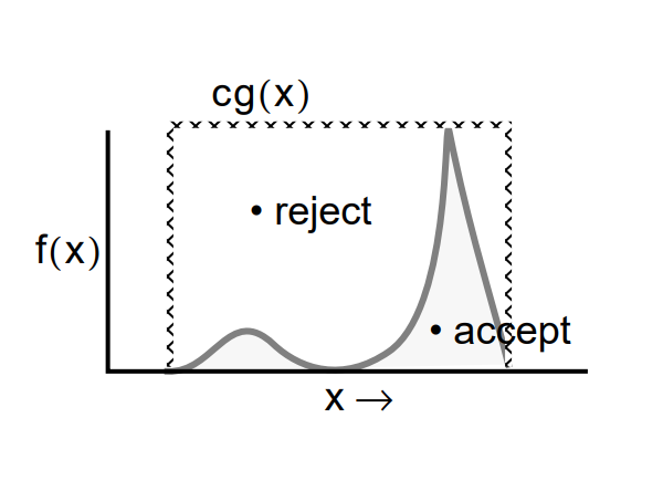
Let f(x) be our distribution that is difficult to sample from. Instead of sampling directly from f(x), we will sample from g(x). Here g(x) may be any well-defined distribution that is easy to sample from like the normal distribution and the uniform distribution.

According to this method, as long as there is a proxy distribution g(x) that can be multiplied by a constant c such that f(x) ≤ c(g(x)) at all times, then we can use a random sample from c(g(x)) to get a random sample from f(x). Here, it is important that the function c(g(x)) envelopes f(x). Now, if our sample is is a part of both the distributions, then we accept it. Else, we reject the sample. Hence, this is also known as the Accept-Reject method.

Steps:

1. Draw random samples x from the 'easy to sample from' distribution g(x).
2. Draw random samples u from the uniform distribution.
3. Accept the random sample x_i if u_i ≤ ( f(x_i) / c(g(x_i)) )
4. Else reject the random sample.

Markov chain Monte Carlo (MCMC) sampling

Metropolis-Hastings algorithm

This algorithm is used when we cannot use any one of the above mentioned techniques (for example, our function f(x) may be difficult to integrate), but we can evaluate f(x) at least upto a normalizing constant or proportionality. Here, we construct and sample from a Markov chain, whose stationary distribution is the target distribution we are looking for.

Let f(x) be out target density and let us assume that we only know it upto a proportionality g(x). The steps for Metropolis-Hastings algorithm is as follows:

1. Select an initial value for x , say x₀.
2. For a large number of iterations where i=1,2,...,m , we repeat the below steps:
   • Draw a sample (say x^* ) from a proposal distribution q(x ^*| x_i-1). We have to be careful while choosing our proposal distribution q. It may or may not always depend on the previous iteration value of x.
   • Calculate the acceptance probability α as
     
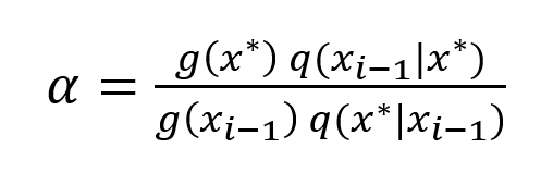
   • If α ≥ 1, then accept x ^* and set x_i ← x ^*.
   • If 0 < α < 1, then either accept x ^* and set x_i ← x ^* with a probability α or reject the candidate and set x_i ← x_i-1 with a probability 1-α.

Here, at each step in the chain, we draw a sample and decide whether to move the chain or not. Since our decision to move to the candidate depends on where our chain currently is, this is a Markov chain.

Gibbs Sampling

This algorithm is a special case of Metropolis-Hastings algorithm where the target distributions are multi-dimensional. In Gibbs sampling, we sample from full conditional distribution arising from the target distribution.

A full conditional distribution of a random vector is the distribution of the random vector conditional on all the other random variables in the target distribution.

Let x be a vector of all random variables in the target distribution p(x|y). x is partitioned into d individual components which may be a random variable or a vector:
x=(x₁,x₂,......,x_d). The notation x_-j denotes the vector containing all the components of x except the j^th component (i.e. x_j).

Now, the full conditional distribution of x_j is denoted as p(x_j|x_-j,y). It is the distribution of the component x_j conditional on knowing the values of all other components (x_-j) and the data y.

The steps in Gibbs sampling is as follows:

1. Choose a vector of starting values for x. ( x⁽⁰⁾=(x₁⁽⁰⁾,x₂⁽⁰⁾,...,x_d⁽⁰⁾) ) .
2. Set the time step t=1.
3. Draw x_j^(t) from the full conditional distribution p(x_j|x_-j^(t-1),y) for j=1,2,...,d where:
   • x_j^(t) denotes the sampled value of x_j in cycle t.
   • x_-j^(t-1) denotes the most current values of all the d components of the vector x except x_j.
4. Increment t.
5. Keep repeating steps 3 and 4 until the Markov chain converges to its stationary distribution.

With this article at OpenGenus, you must have the complete idea of different Monte Carlo Sampling Techniques in Data Science.