
We are now in the last part of the ShuffleNet series. I have already introduced the ShuffleNet family and we have seen the power of ShuffleNet in my previous articles. This article will include the complete explanation of building ShuffleNet using Pytorch, a popular deep learning package in Python. I will be covering the step by step tutorial starting from installation of all required packages to testing the Shufflenet model and visualization using CIFAR 10 dataset. We are going to build a multi-class image classifier which has an overall average accuracy of 85.37%.
As a bonus section, which is a very crucial step, I am going to cover the discussion of results obtained after evaluating the model.
One can follow the same tutorial for 3 different platforms; Google Colab, Kaggle as well as Local Jupyter Notebook using Anaconda or any python environment providing softwares.
Table of Contents
- Introduction of Dataset
- Implementation of Shufflenet V1 using Python
2.1 Setup & Importing libraries
2.2 Initializing Constants
2.3 Exploring Dataset
2.4 Loading Dataset with Data Augmentation
2.5 Creating ShuffleNet Network
2.6 Setting up loss function and optimizer
2.7 Loss Accuracy Calculation
2.8 Defining training method
2.9 Saving best model
2.10 Model Training - Results and Discussion
3.1 Evaluation of Model and Results
3.2 Plotting confusion matrix
3.3 Understanding confusion matrix results and created model [CRITICAL SECTION]
Introduction of Dataset
CIFAR 10 dataset is a labeled dataset of 60,000 color images of 32 X 32 size. This dataset is a subset of 80 million tiny images. The images belong to 10 classes of objects, namely airplane, car, bird, cat, deer, dog, frog, horse, ship and truck. The classes are mutually exclusive and hence, each image belong to only one class.
Out of the 60,000 images, 50,000 are in training set and rest 10,000 are in test set. The training set consists of 5 unequal batches with 5000/class and test set has 1000 randomly selected images per class. We will be using this dataset as such after downloading from its source without any data cleaning. However, we will be performing some data augmentation techniques, which will be discussed later in this article.
Implementation of Shufflenet V1 using Python
The following is a 10 step methodology for building the multi-class classifier. I have followed an object oriented approach for creating the model. The steps have to be followed sequentially for replicating the same results. I will be using a Jupyter notebook since it is easy to share and provides efficient modularity. But, the same can be performed using a simple single Python file, or a set of python files if modularity is what you want.
As mentioned, one can follow this tutorial for 3 platforms, so I will be giving specific instructions for Kaggle, Google Colab and Local Notebook wherever needed. The steps where specific instructions are not given are common for all three platforms. I personally suggest using Kaggle due to its longer GPU usage support as compared to Colab.
Step 1: Setup & Importing libraries
a) Setup
Let's first talk about the computational specifications.
The training of a deep learning model is a computationally expensive job. So, it is better to use an environment which is GPU enabled. With that said, it is NOT mandatory to have access to GPU and training happens comfortably (but takes longer time) without GPU too. I usually start training the model, go have lunch or complete my daily workout and my training is done by the time I am back!! You can do the same.
Now, the second important aspect for setting up is the packages that need to be installed.
For Local Jupyter Notebook
The following packages have to be installed for the ones working on local jupyter notebook using anaconda or pip.- Pytorch, preferably cuda enabled - for model architecture creation, data augmentation, data loader, optimizer, training and testing
- numpy - for all matrix operations
- os - for saving and loading checkpoint
- math - for math operations
- datetime - for finding time of training
- tqdm - for loader
- tarfile - for unzipping dataset
- warnings - for disabling warnings
- matplotlib - for plotting images
- PIL - for image processing
For Google Colab/ Kaggle
These packages are already installed in the working session and only need to be imported for usage. The following code shows the same.b) Importing required libraries
Next, one has to import all these required libraries.
import torch
import torch.nn as nn
import torchvision.transforms as transforms #for data augmentation; here, image transformations
import torchvision.datasets as dsets #for data loaders for popular vision datasets
from torchvision import  models #for definitions for popular model architectures
from torchsummary import summary #to get model summary after declaring it
from torch import nn,optim
import torch.nn.functional as functions #for non linear functions
import torchvision

import numpy as np
import pandas as pd

#core python packages
import os
import sys
import time
import math
import datetime as dt
import tqdm
import tarfile
import warnings
warnings.filterwarnings("ignore")

#for plotting images
import matplotlib.pyplot as plt
from PIL import Image
Step 2: Initializing Constants
Before we begin defining models and getting the dataset, we need to declare some contant variables that would be used accross the whole project. Comments and names for each constant are self explanatory.
device = 'cuda' if torch.cuda.is_available() else 'cpu' #to set the device to be used by pytorch
best_acc = 0 #best test accuracy
start_epoch = 0 #start from epoch 0 or last checkpoint epoch
batch_size = 128
weight_decay = 5e-4
momentum = 0.9
learning_rate = 0.01
epoch_size = 60

#declaring constant label mapper for CIFAR 10 dataset
LABEL_MAP = {0:'airplane', 1:'car', 2:'bird', 3:'cat', 4:'deer', 5:'dog', 6:'frog', 7:'horse', 8:'ship', 9:'truck'}
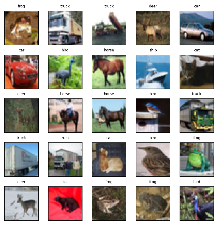
Step 3: Exploring Dataset
Now, let's look into our dataset to get an insight on how the images are. This is a crucial part of any data science project too. We're using matplotlib for the same. The output follows the code. We can observe that these are colour images hence we have 3 channels (R, G and B). The images are of a considerable low quality but it is enough to extract features and notice patterns for our CNN. You can explore further and look into the shape of the train and test data.
from matplotlib.pyplot import figure
figure(num=None, figsize=(5, 5), dpi=150, facecolor='w', edgecolor='k')

#Exploring image dataset
def show_imgs(X):
  plt.figure(1)
  plt.rcParams.update({'font.size': 5})
  k=0
  for i in range(0,5):
    for j in range(0,5):
      plt.subplot2grid((5,5),(i,j))
      plt.title(LABEL_MAP[X[k][1]])
      plt.imshow(X[k][0])
      plt.tick_params(axis='x', which='both', bottom=False, top=False, labelbottom=False)
      plt.tick_params(axis='y', which='both', left=False, right=False, labelleft=False)
      k = k+1
  #show the plot
  plt.tight_layout()
  plt.show()

data_train = dsets.CIFAR10(root=root_path, download = True)
data_test = dsets.CIFAR10(root=root_path, download=True, train=False)
show_imgs(data_train)
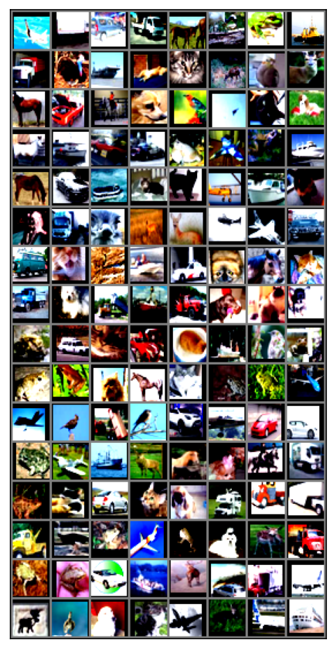
Step 4: Loading Dataset with Data Augmentation
After exploration, we'll be loading the dataset using pytorch's dataset module. Next, we have to perform some data augmentation tasks to make our classifier robust. I have performed random horizontal flip and random crop of each image. You can also try doing vertical flip, changing jitter,saturation of the image and even making it grayscale. Next, all the images are normalized by subtracting the mean and dividing the standard deviation. This is performed to ensure a similar data range distribution across all channels and thus helps in convergence of our model. If you want to read more about it, I have left a link in the references for the same.
To support our convoluted image dimensions, we have to add a padding of 4. Additionally, since we have used pytorch and wish to work on tensors in the next steps. Thus, I have used a ToTensor transformation to convert them to tensors.
To conclude, we have performed 4 transformations which have 2 data augmentation tasks, namely random horizontal flip and random crop, a model requirement namely adding padding and a programming requirement, namely conversion to tensor.
Remember that during testing, we'll be doing the same transformations to the test images as our classifier has been trained on such transformed images. You can notice that the images look more darker in Figure 2.
#defining transformation rules for training set
transform_train = transforms.Compose(transforms=[transforms.Pad(4), transforms.RandomHorizontalFlip(), transforms.RandomCrop(32), transforms.ToTensor(), transforms.Normalize((0.4914, 0.4822, 0.4465), (0.2023, 0.1994, 0.2010))])

#defining transformation rules for testing set
transform_test = transforms.Compose(transforms=[transforms.ToTensor(), transforms.Normalize((0.4914, 0.4822, 0.4465), (0.2023, 0.1994, 0.2010))])

train_set = dsets.CIFAR10(root=root_path, download = True, transform= transform_train)
train_loader = torch.utils.data.DataLoader(train_set, batch_size=batch_size, shuffle=True, num_workers=2)

test_set = dsets.CIFAR10(root=root_path, download=True, train=False, transform= transform_test)
test_loader = torch.utils.data.DataLoader(test_set, batch_size=batch_size, shuffle=False, num_workers=2)

#looking into the transformed images
figure(num=None, figsize=(10,8), dpi = 150, facecolor = 'w', edgecolor='k')
def imshow(img):
  img = img/2 + 0.5 #unnormalize
  np_img = img.numpy()
  plt.imshow(np.transpose(np_img, (1,2,0)))
  plt.tick_params(axis='x', which='both', bottom=False, top=False, labelbottom=False)
  plt.tick_params(axis='y', which='both', left=False, right=False, labelleft=False)
  plt.show()

#get random training example images
data_iter = iter(train_loader)
images, labels = data_iter.next()

#understanding image tensor
images[0].shape

#show images
imshow(torchvision.utils.make_grid(images))
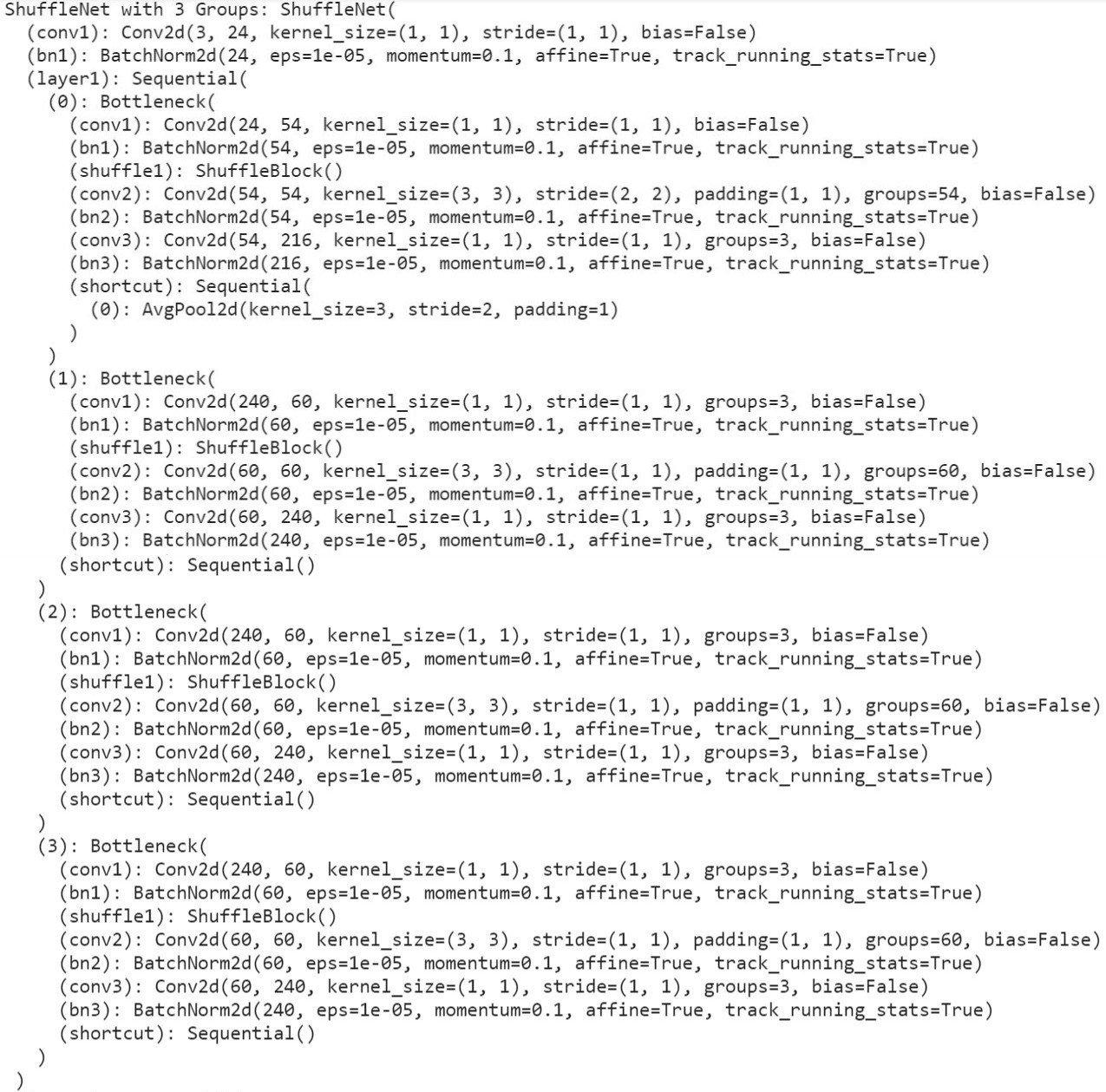
Step 5: Creating ShuffleNet Network
Let's define the ShuffleNet model by taking reference of the layers from the official paper shown in figure 1. I have created 5 classes for the same. The ShuffleBlock defines the blueprint of the each ShuffleNet operation. Bottleneck is the residual network block that involves 3 grouped convolutions with shuffle operation after the first convolution. All the grouped convolutions are followed by a batch normalizer. Now, the structure varies slightly for stride 1 and 2 in the shortcut connection. Stride 2 has an average pool operation whereas stride 1 is a simple direct shortcut connection. Each batch normalization is followed by a ReLU activation. ShuffleNet brings all this together.
I have initialized two ShuffleNet networks ShuffleNetG2 and ShuffleNetG3 which differ at no of groups as the names suggest. I have gone forward with groups = 3 since it has proved to work the best. I have tried with both groups as 2 and 3 and for this task, groups = 3 works better. As an exercise, you can go ahead and try with groups=2.
After defining the network, we have to put the network onto the device, be it CPU or CUDA. It is important to note that we have to keep everything on the same device for the model to train.
A section of structural summary of our model can be seen in the output following the code snippet.
class ShuffleBlock(nn.Module):
  def __init__(self, groups):
    super(ShuffleBlock, self).__init__()
    self.groups = groups
  def forward(self, x):
    N,C,H,W = x.size()
    g = self.groups
    return x.view(N, g, C//g, H, W).permute(0, 2, 1, 3, 4).reshape(N, C, H, W)
class Bottleneck(nn.Module):
  def __init__(self, in_planes, out_planes, stride, groups):
    super(Bottleneck, self).__init__()
    self.stride = stride
    mid_planes = int(out_planes/4)
    g = 1 if in_planes == 24 else groups
    self.conv1 = nn.Conv2d(in_planes, mid_planes, kernel_size=1, groups=g, bias=False)
    self.bn1 = nn.BatchNorm2d(mid_planes)
    self.shuffle1 = ShuffleBlock(groups= g)
    self.conv2 = nn.Conv2d(mid_planes, mid_planes, kernel_size=3, stride=stride, padding=1, groups=mid_planes, bias=False)
    self.bn2 = nn.BatchNorm2d(mid_planes)
    self.conv3 = nn.Conv2d(mid_planes, out_planes, kernel_size=1, groups=groups, bias=False)
    self.bn3 = nn.BatchNorm2d(out_planes)
    self.shortcut = nn.Sequential()
    if stride==2:
      self.shortcut = nn.Sequential(nn.AvgPool2d(3,stride=2, padding =1))
  def forward(self,x):
    out = functions.relu(self.bn1(self.conv1(x)))
    out = self.shuffle1(out)
    out = functions.relu(self.bn2(self.conv2(out)))
    out = self.bn3(self.conv3(out))
    res = self.shortcut(x)
    out = functions.relu(torch.cat([out,res], 1)) if self.stride==2 else functions.relu(out+res)
    return out
class ShuffleNet(nn.Module):
  def __init__(self, cfg):
    super(ShuffleNet, self).__init__()
    out_planes = cfg['out_planes']
    num_blocks = cfg['num_blocks']
    groups = cfg['groups']
    self.conv1 = nn.Conv2d(3, 24, kernel_size=1, bias = False)
    self.bn1 = nn.BatchNorm2d(24)
    self.in_planes = 24
    self.layer1 = self._make_layer(out_planes[0], num_blocks[0], groups)
    self.layer2 = self._make_layer(out_planes[1], num_blocks[1], groups)
    self.layer3 = self._make_layer(out_planes[2], num_blocks[2], groups)
    self.linear = nn.Linear(out_planes[2], 10) #10 as there are 10 classes

  def _make_layer(self, out_planes, num_blocks, groups):
    layers = []
    for i in range(num_blocks):
      stride = 2 if i == 0 else 1
      cat_planes = self.in_planes if i==0 else 0
      layers.append(Bottleneck(self.in_planes, out_planes-cat_planes, stride=stride, groups=groups))
      self.in_planes = out_planes
    return nn.Sequential(*layers)

  def forward(self,x):
    out = functions.relu(self.bn1(self.conv1(x)))
    out = self.layer1(out)
    out = self.layer2(out)
    out = self.layer3(out)
    out = functions.avg_pool2d(out, 4)
    out = out.view(out.size(0), -1)
    out = self.linear(out)
    return out
def ShuffleNetG2():
  cfg = {'out_planes': [200, 400, 800],
         'num_blocks': [4, 8, 4],
         'groups': 2
         }
  return ShuffleNet(cfg)

def ShuffleNetG3():
  cfg = {'out_planes': [240, 480, 960],
         'num_blocks': [4, 8, 4],
         'groups': 3
         }
  return ShuffleNet(cfg)

#Shufflenet with groups = 2
net2 = ShuffleNetG2()
print("ShuffleNet with 2 Groups: " + str(net2))

#Shufflenet with groups = 3
net3 = ShuffleNetG3()
print("ShuffleNet with 3 Groups: " + str(net3))
#we will be using g=3 for training

#Setting the model with CUDA
if torch.cuda.is_available():
  net3.cuda()
Step 6: Setting up loss function and optimizer
The loss function we'll be using is cross entropy loss and a stochastic gradient descent optimizer. All the constant values of the parameters were previously defined in initializing constants section.
criterion = nn.CrossEntropyLoss()
optimizer = optim.SGD(net3.parameters(), lr = learning_rate ,momentum= momentum, weight_decay=weight_decay)
Step 7: Loss Accuracy Calculation
Next, we define a function for calculating loss accuracy by adding up all correct predictions. The dataloader here, if set to be training set, then we'll be calculating validation accuracy. But in that case, we need to send only a part of train set, or else it'll be train loss.
def get_loss_acc(is_test_dataset = True):
  net3.eval()
  dataloader = test_loader if is_test_dataset else train-loader
  n_correct = 0
  n_total = 0
  test_loss = 0
  with torch.no_grad():
    for batch_size, (inputs, targets) in enumerate(dataloader):
      inputs, targets = inputs.to(device), targets.to(device)
      outputs = net3(inputs)
      test_loss += criterion(outputs, targets).item()
      _, predicted = outputs.max(1)
      n_correct +=predicted.eq(targets).sum().item()
      n_total += targets.shape[0]

  return test_loss/(batch_size+1), n_correct/n_total
Step 8: Defining training function
Now, let's define the training function. For each batch, we traverse through our training set to run our ShuffleNet (with groups=3) model, get the outputs, find loss using loss method defined, do back propagation to get derivatives and lastly update weights. This process is constant for all training methods. Next, I have found training loss in a similar way as loss accuracy calculation.
def train_model():
  net3.train()
  train_loss = 0
  n_correct = 0
  n_total = 0
  for batch_size, (inputs, targets) in enumerate(train_loader):
    inputs, targets = inputs.to(device), targets.to(device)
    optimizer.zero_grad()
    outputs = net3(inputs)
    loss = criterion(outputs, targets)
    loss.backward()
    optimizer.step()
    train_loss += loss.item()
    _, predicted = outputs.max(1)
    n_correct +=predicted.eq(targets).sum().item()
    n_total += targets.shape[0]
  return train_loss/(batch_size+1), n_correct/n_total
Step 9: Saving best model
Just before we set up our training, lets define the method for saving the best model. We'll be keeping our best accuracy as a global variable and use it to compare all newly calculated accuracies during each epoch. If the new accuracy is the best one, we'll be making the new accuracy as the best one and save the model and optimizer state for loading it in future.
def save_best_model(epoch):
  global best_acc
  net3.eval()
  test_loss = 0
  correct = 0
  total = 0
  with torch.no_grad():
    for batch_idx, (inputs, targets) in enumerate(train_loader):
      inputs, targets = inputs.to(device), targets.to(device)
      outputs = net3(inputs)
      loss = criterion(outputs, targets)
      test_loss += loss.item()
      _, predicted = outputs.max(1)
      total += targets.size(0)
      correct +=predicted.eq(targets).sum().item()
      print(batch_idx, len(train_loader), 'Loss: %.3f | Acc: %0.3f%% (Correct classifications %d/Total classifications %d)' % (test_loss/(batch_idx+1), 100.*correct/total, correct, total))

      #save checkpoint
      acc =100.*correct/total
      if acc>best_acc:
        print('Saving...')
        state = {'net': net3.state_dict(),
                 'acc': acc,
                 'epoch': epoch
                 }
        if not os.path.isdir('checkpoint'):
          os.mkdir('checkpoint')
        torch.save(state, './checkpoint/ckpt.pth')
        torch.save(net3, './checkpoint/net3.pth')
        best_acc = acc
Step 10: Model Training
Now here's the most dreaded step! THE TRAINING ...
We iterate through the no of epochs to train weights in our ShuffleNet. Rest of the code is self explanatory. Additionally, I have calculated the total training time using datetime module.
My training took 2 hours 22 minutes and 73 seconds. I had trained using Google Colab with GPU enabled. If your configuration doesn't have GPU that it will probably take the double amount.
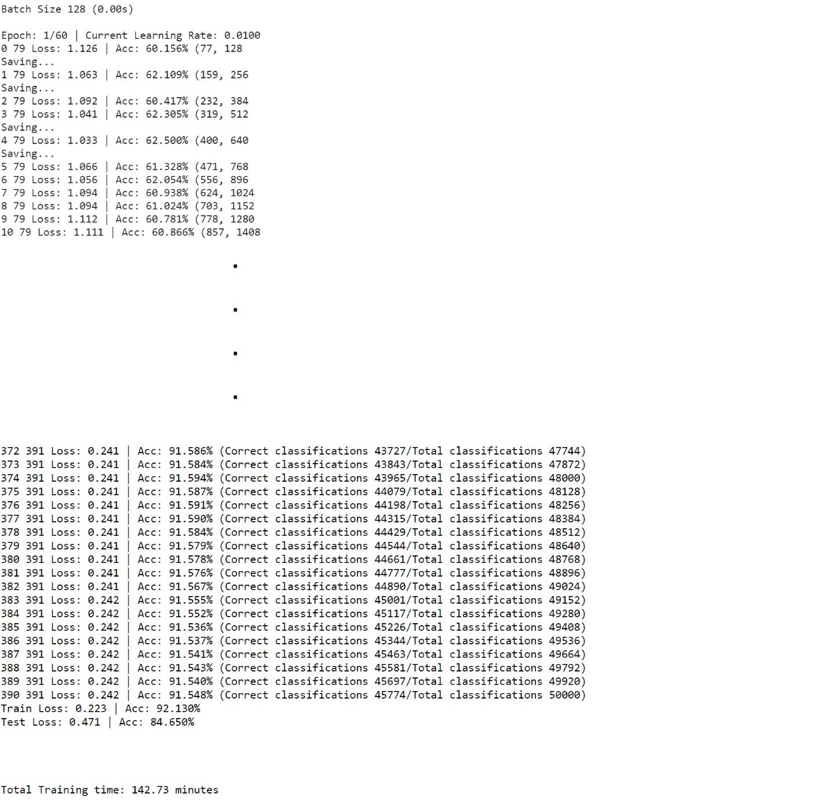
A small glimpse of how the output looks like is under the code snippet. It repeats until all the epochs are completed.
EPOCH = epoch_size
training_time = dt.datetime.now()
start = dt.datetime.now()
start_epoch = 0
train_accuracy_list = []
test_accuracy_list = []
for epoch_i in range(start_epoch, start_epoch + EPOCH):
  global accuracy_list
  current_learning_rate = [i['lr'] for i in optimizer.param_groups][0]
  print('Batch Size', batch_size, '(%0.2fs)\n\nEpoch: %d/%d | Current Learning Rate: %.4f ' % ((dt.datetime.now() - start).seconds, epoch_i +1, EPOCH+start_epoch , current_learning_rate))
  start = dt.datetime.now()
  test_loss, test_acc = get_loss_acc()
  train_loss, train_acc = train_model()
  train_accuracy_list.append(train_acc*100)
  test_accuracy_list.append(test_acc*100)
  save_best_model(epoch_i)
  print('Train Loss: %.3f | Acc: %.3f%% \nTest Loss: %0.3f | Acc: %0.3f%% \n\n' % (train_loss, train_acc*100, test_loss, test_acc*100))

print('\n\nTotal Training time: %0.2f minutes ' %((dt.datetime.now() - training_time).seconds/60))
Results and Discussion
Now, since the most time-consuming task is done, we can test our model on our test set. This is the most exciting part!! Aleast for me..
So, we'll start with evaluation of our model and look at how well it predicts unknown and unseen images. Fingers crossed. Then, we'll be plotting the confusion matrix for this classifier which is like the exam result card of our whole training process. And at last we'll be understanding our exam card and the model that we spent so much time training!
Evaluation of Model and Results
Let's test the model on our training set which contains 1000 randomly selected images of all classes. We calculate our confusion matrix that is a 10 X 10 matrix that contains the classes that the predicted images were put into and the original class of the image. This helps in understanding incorrect classifications. With that we are also calculating accuracy of correctly classifying each class by dividing correct classifications by total classifications. Following the code snippet is a subset of the testing results.
Note: All images are normalized for testing, remember to un-normalize it while plotting.
Note: Testing happens without any gradient calculation or parameter updations, hence it is necessary to perform the whole process with torch.no_grad().
class UnNormalize(object):
def __init__(self, mean, std):
self.mean = mean
self.std = std
def __call__(self, tensor):
for t, m, s in zip(tensor, self.mean, self.std):
t.mul_(s).add_(m)
# The normalize code -> t.sub_(m).div_(s)
return tensor
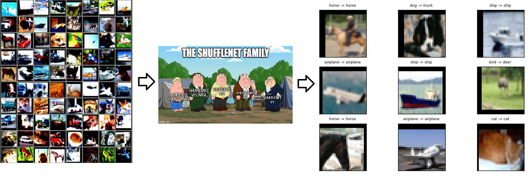
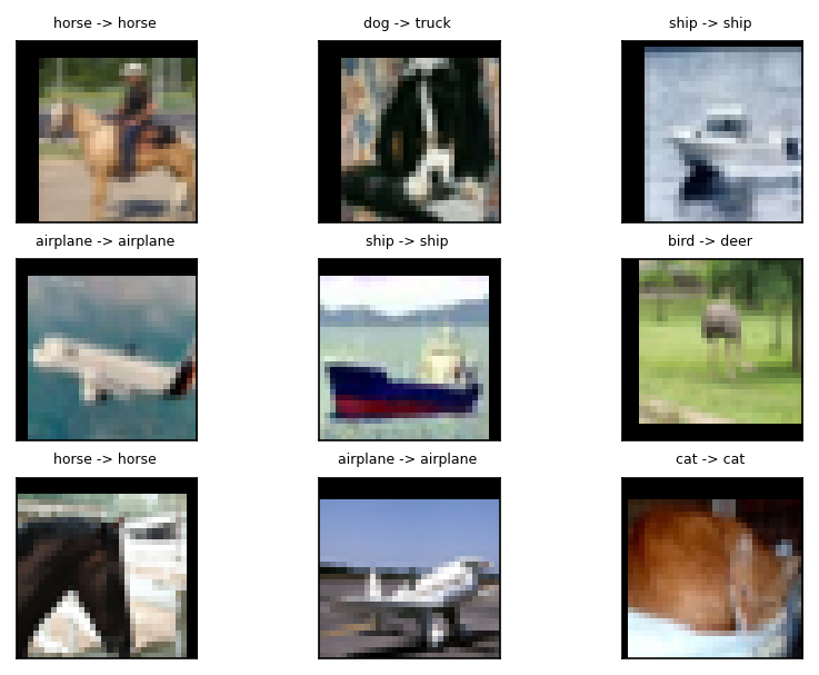
#seeing predictions of some images
def show_test_prediction_imgs(images, predicted_labels, real_labels):
plt.figure(1, dpi = 150)
plt.rcParams.update({'font.size': 5})
k=0
for i in range(0,3):
for j in range(0,3):
plt.subplot2grid((3,3),(i,j))
plt.title('{0} -> {1} '.format(LABEL_MAP[real_labels[k].item()],LABEL_MAP[predicted_labels[k].item()]))
unorm = UnNormalize(mean=(0.4914, 0.4822, 0.4465),std = (0.2023, 0.1994, 0.2010))
image = unorm(images[k].cpu())
plt.imshow(np.transpose(image.numpy(), (1,2,0)))
plt.tick_params(axis='x', which='both', bottom=False, top=False, labelbottom=False)
plt.tick_params(axis='y', which='both', left=False, right=False, labelleft=False)
k = k+1
#show the plot
plt.tight_layout()
plt.show()
#Model Accuracy
total_correct = 0
total_images = 0
confusion_matrix = np.zeros([10,10], int)

with torch.no_grad():
  for i,data in enumerate(test_loader):
    images, labels = data
    images, labels = images.to(device), labels.to(device)
    outputs = net3(images)
    _, predicted = torch.max(outputs.data, 1)
    if(i in [0,1]):
      show_test_prediction_imgs(images, predicted, labels)
    total_images += labels.size(0)
    total_correct += (predicted == labels).sum().item()
    for i, l in enumerate(labels):
      confusion_matrix[l.item(), predicted[i].item()] +=1
Plotting confusion matrix
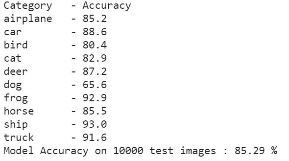
Now, lets look at the confusion matrix created to get the accuracies of each class. Then, the model accuracy is also calculated.
print('{0:10s} - {1}'.format('Category', 'Accuracy'))
for i, r in enumerate(confusion_matrix):
  print('{0:10s} - {1:0.1f}'.format(LABEL_MAP[i], r[i]/np.sum(r)*100))
model_accuracy = total_correct/total_images *100
print('Model Accuracy on {0} test images : {1:.2f} %'.format(total_images, model_accuracy))
Confusion matrix is best understood when plotted as a matrix plot with colors depicting the value. The following is the code for the same and following that is the plotted matrix.
    fig, axis = plt.subplots(1,1,figsize = (10,10))
axis.matshow(confusion_matrix, aspect='auto', vmin = 0, vmax = 1000, cmap= plt.get_cmap('Wistia'))
for (i, j), z in np.ndenumerate(confusion_matrix):
  axis.text(j, i, '{:0.2f}'.format( z/np.sum(confusion_matrix, 0)[i]*100), ha='center', va='center')
plt.ylabel('Actual Category')
plt.yticks(range(10), LABEL_MAP.values())
plt.xlabel('Predicted Category')
plt.xticks(range(10), LABEL_MAP.values())
plt.rcParams.update({'font.size': 14})
plt.show()
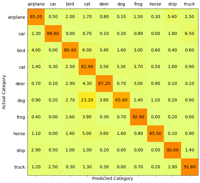
Understanding confusion matrix results and created model [CRITICAL SECTION]
Having seen the accuracies and confusion matrix, we can make some prominent conclusions about our classifier. But before that let's understand the importance of this section. Gaining insights from the results is key to understand the model. This helps us in noting down what works for image classifiers, what features the model learns and further helps us get an idea on where it is lagging.
ANALOGY TIME
Taking the analogy of an exam, training is like teaching a student and testing is examination taken by the student. Now, after the test, introspection and reflection on the results decides how well you will perform in the next test in the same subject. It is important to understand what went well, what the student didn't understand and that helps the teacher and student to understand what steps have to be taken to improve the exam results.
Now that we have understood the prominence of this step, let's take a look at key observations and talk about it in depth.
-
It gives impressive results
As all the 10 classes are predicted correctly with more than 75% accuracy on the training set, we can say that our model performs well. Kudos to us for creating such a well performing classifier!👏🏽 -
The trained ShuffleNet is best at recognizing a ship and is worst at identifying a cat!
The highest accuracy i.e. 95% is for frog and the lowest i.e. 72.4% is for cat. Note that the reason for highest accuracy also means that there are least mis-classifications of frog as compared to any other class. Our confusion matrix plot proves the same; see the row (not column) for frog. A reason for this could be the absence of any classes that look like a frog. If the dataset had images of toads then this class might not have been the best.
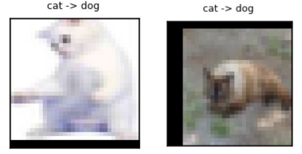
Likewise, cats have very high structural similarity with dogs. Hence, the model was unable to differentiate between them leading to incorrect classifications as dogs for cat images. Another point to note is the mis-classification of cat as a bird and frog but not vise-e-versa. The reason for this could be unavailability of cat images in different lightening conditions or angles. With more data for cat category, we could improve its accuracy. -
It is greatly confused between dog and a cat
A big observation looking at our confusion matrix is cat being mis-classified as dog and vise-e-versa with as high as 10% accuracy. This is a very faulty case. As stated above, the reason for this is the similarity in dog and cat in terms of color, height and surroundings where it is found. We can control the mis-classification by including more cat pictures in different angles and types of cats.
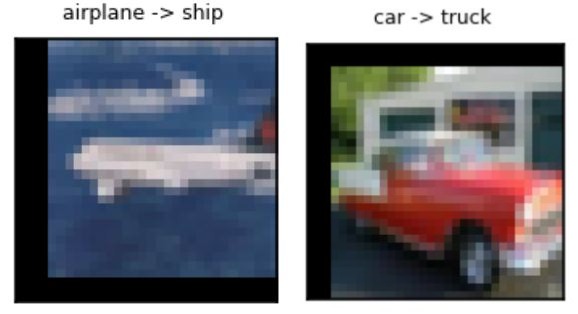
- Some of the mis-classifications are among the same higher-level group of objects
By higher level groups, I mean animals and vehicles. As per the confusion matrix, we can see that dogs and cats are undifferentiable for our classifier. A similar case is seen in car and truck. The major cause for this is the same, the pixels around the car and truck would usually be roads or people. Ships and aeroplanes also share blue colored sky(for aeroplanes) and water(for ships) in nearby pixels to the object. Their structure shape and colors are also usually similar. To rectify this issue we can either get more data or train it for more epochs.
Another perspective is; this misclassification is actually good! We now know where our data lags and can rectify it. Also, we understood the classifiers main criteria for distinguishing.
-
Some of the mis-classifications are fairly reasonable
Our model confuses birds as aeroplanes and vise-e-versa. The most obvious reason for this is both have wings, body shape, both move in sky and their flying position. The sitting bird wouldn't have been confused as an aeroplane as much as a flying one. Cars being misclassified as ships are usually white in color. Other such similarities can be understood by looking at the images.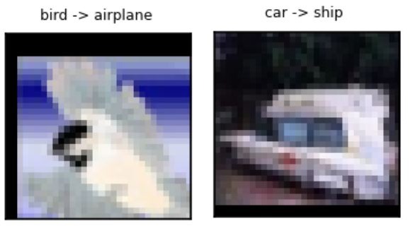
Figure 10: Reasonable misclassification
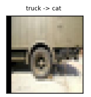
- Few of the mis-classifications are impractical for us!
There are a few mis-classifications which couldn't be explained. The sole reason for this and can be improved by increasing data and training it.
Conclusion
We have covered every step involved in training and testing our ShuffleNet model in 3 different platforms including Kaggle, Google Colab and Local Jupyter Notebook that performs multi-class image classification. We started out with introduction of dataset, then looked into step by step tutorial and completed it with testing and result discussion. We also understood that understanding the trained model holds the most significance and should never be skipped.
You can find the entire code on my GitHub repository
Outro
This article is the last in the series. I had a lot of fun researching, understanding and writing about the ShuffleNet family. Although implementing the model by coding it seems to be the most visually appealing section as we can see the output of our classifier but trust me understanding the model is what makes the implementation simple.
See you people with another architecture! Happy (deep) learning :)
References
- In-depth Explanation about ShuffleNet family :ShuffleNet Series (Part 1)
- Comparison with popular models including VGG 16, GoogleNet, MobileNet, etc. :ShuffleNet Series (Part 2)
- Learning Multiple Layers of Features from Tiny Images, Alex Krizhevsky, 2009.