
Let's begin
With the advent of Edge AI, researchers have been keen to look into fast, accurate, memory-efficient, computationally cheap and reliable algorithms for edge devices including mobile phones, drones, surveillance and monitoring cameras, autonomous cars and various other smart Internet of Things(IOT) enabled devices. Megvii is a Chinese AI powered tech company which is the largest provider of third-party authentication software in the world. It's product, Face++ is a computer vision enabled face-detection tool (now, extended to body recognition and image detection and beautification) is used by millions accross the world.
ShuffleNet was pioneered by Xiangyu Zhang et al. for the same.
Table of Contents
This article consists of the following sections and covers everything one needs to know about ShuffleNet.
- What is ShuffleNet & its siblings?
- When did ShuffleNet come into picture?
- Meet the ShuffleNet family!
- Which operations make the core of ShuffleNet?
- Other similar architectures
What is ShuffleNet & its siblings?
ShuffleNet is simple yet highly effective CNN architecture which was contrived specially for devices with low memory and computing power, i.e. 10-150 MFLOPs(Mega Floating-point Operations Per Second). It became highly popular due to its outstanding experimental results and hence top universities have included it in their coursework. Many algorithms inspired or closely related to this have been mentioned in the Other similar Architectures section of this article.
Following that, ShuffleNet V2 was presented by Ningning Ma et. al. from Megvii and Tsinghua University which examines other indirect metrics (here, MFLOP's are direct metrics) like Memory Access Cost (MAC), degree of parallelism and platform dependency. They propose new guidelines for a much faster and more accurate network structure for mobile devices that works seamlessly on both GPU as well as ARM based devices.
The newest versions of ShuffleNet including ShuffleNetV2 Large and ShuffleNet V2 Extra Large architectures are deeper network with higher trainable parameters and FLOP's to support devices with higher computing as well as storage power.
Meet the ShuffleNet Family!
The following is a brief introduction to all the members of the ShuffleNet family as mentioned on its official link:
- ShuffleNetV1: ShuffleNet: An Extremely Efficient Convolutional Neural Network for Mobile Devices
- ShuffleNetV2: ShuffleNet V2: Practical Guidelines for Efficient CNN Architecture Design
- ShuffleNetV2+: A strengthen version of ShuffleNetV2.
- ShuffleNetV2.Large: A deeper version based on ShuffleNetV2 with 10G+ FLOPs.
- ShuffleNetV2.ExLarge: A deeper version based on ShuffleNetV2 with 40G+ FLOPs.
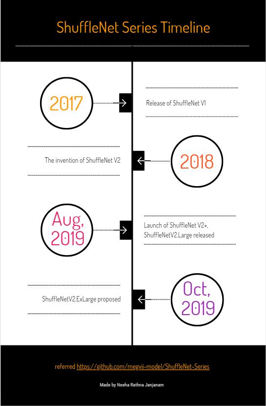
When did ShuffleNet come into picture?
The following infographic timeline gives an idea about the inventions of all versions and variations of ShuffleNet.
Which operations make the core of ShuffleNet?
ShuffleNet V1
The architecture of ShuffleNet is inspired by three pioneering CNN architectures; GoogleNet for its group convolution, ResNet for its skip connections and Xception for its depthwise separable convolutions. ShuffleNet proposes a group convolution of pointwise convolutions with a residual shortcut path based structure.
1. Grouped Pointwise Convolution
First let me brief about Group Convolution. Group Convolution, which was introduced in GoogLeNet strives for efficient convolution operation by dividing the filter banks as well as corresponding feature map into groups for processing. This helps in convolution of each group on different GPU's, thus enabling parallel processing. Not only does it speed up the training process but the model ends up learning better representation of the input data. This can be understood in Deep Roots paper.
The model smartly divides convolution into two separate and distinct tasks: black and white filters and color filters for 2 groups. The following figure gives an idea about Group Convolution. One can divide filters into more than 2 groups too.

Image Courtesy: https://blog.yani.ai/filter-group-tutorial
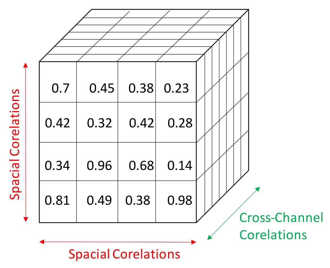
Putting that on hold, the second architecture is Xception.
It introduced depthwise separable convolutions that drastically reduced the number of trainable parameters by separating the spacial and cross-channel correlations(Figure 3). This is done by performing two operations in conjugation; depth-wise convolution and pointwise convolution. Depth-wise convolution involves spacial convolution operation by filters for each channel separately. This forms the intermediate output. Next, a pointwise convolution is performed where a filter of dimension 1X1XC, where C is the number of channels is convolved on the intermediate output. This ensures huge reduction in tunable parameters and hence saves computation power and speed.
Now, authors of ShuffleNet observed that pointwise (1X1XC filter) convolutions are the most computationally heavy operations. It wouldn't be worrisome for large devices but for tiny devices tackling this cuts back a lot of time and computation. They propose a blend of both group convolution and depthwise separable convolution by performing group convolution on pointwise convolutions.
This shows an amazing time gain with not much harm to accuracy. In addition to that, there is a skip connection to avoid vanishing/exploding gradient problem.
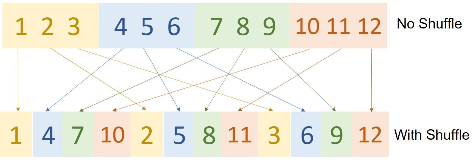
2. Shuffle Operation
A key observation with the grouped pointwise convolution setup is that multiple group convolutions stacked one after other causes outputs of certain channels to be derived from only certain channels. For eg., if there are 4 groups each with 3 channels then the output after pointwise convolution of say 1st group will consist of representations limited to only 1st group and not the others. ShuffleNet authors state that this property blocks information flow between channel groups and weakens representation. To tackle this, they have presented the Shuffle operation that jumbles up the channels across groups.
This shuffling doesn't happen randomly, Figure 4 specifies the steps with an example. Here, G is the number of groups and n is the number of channels in each group. Each group is represented by a different color for visualization of the shuffling operation.
Shuffle operation merges features across channels which strengthens representations. Another advantage of channel shuffle operation is its differentiability.
This means that we don't need to remove it from the network during back propagation. Differentiation of Transpose operation is given as follows:
d (XT) = (d X)T where X represents a matrix and XT represents transpose of the matrix X
The diagram(Figure 6) depicts a typical ShuffleNet with both pointwise group convolution and channel shuffle operation in a skip connection network. The left one shows the network with stride=1, the right one has stride=2 and concat operation to support the dimensions of output feature representations. It consists of two pointwise operations, the second one is done to match the dimension with the skip connection. The shuffle operation for the second pointwise convolution isn't performed as it gives comparable results when shuffle operation is performed. Figure 7 gives an in-depth overview of the entire network architecture of ShuffleNet. Here, Stage 2 and so on have same structure as ShuffleNet unit except Stage 2. Stage 2 has missing group convolution on the first pointwise layer due to small feature space.
For stride=2, two modifications are done-
-
3X3 average pooling is added on skip connection path to consider spacial activations of feature vector through average pooling that might get lost in the Depth Convolution with stride=2.
-
Concatenation operation is done instead of simple addition to enlarge channel dimension with minimal computation cost.
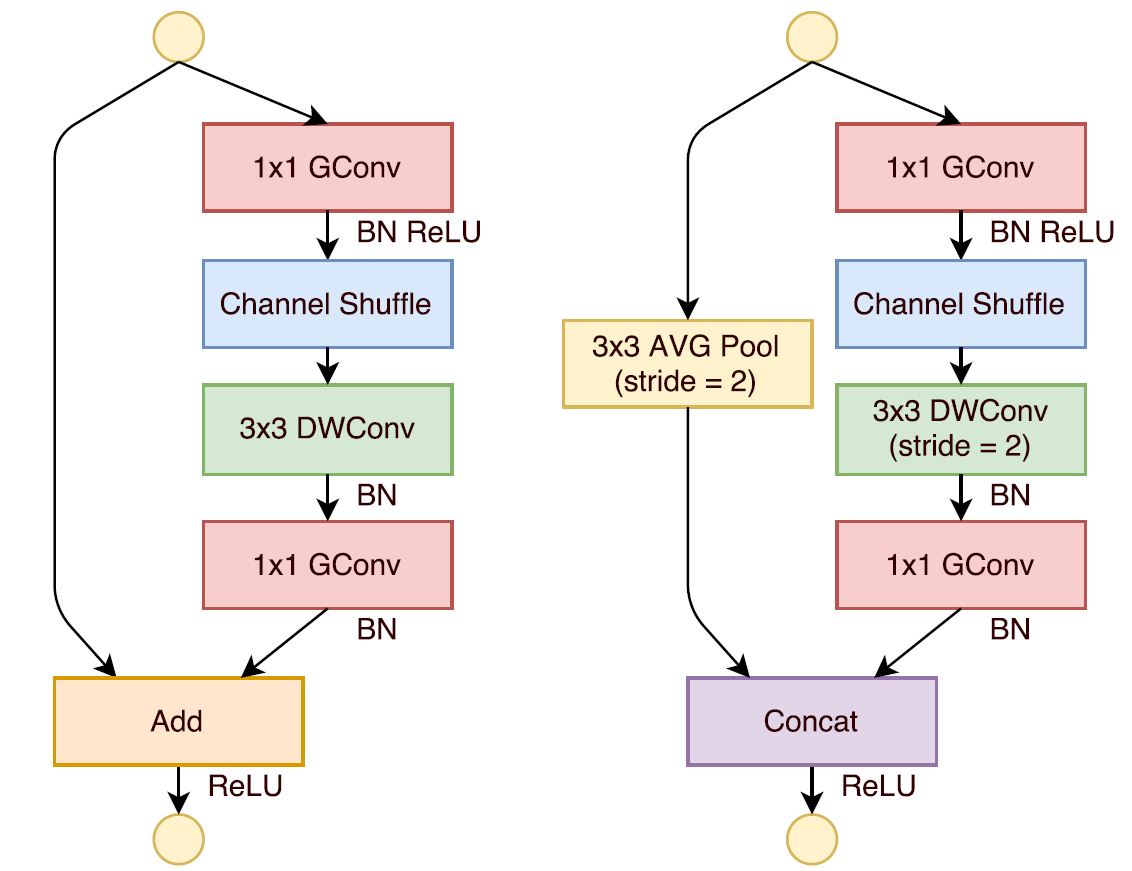
Image Courtesy: Official ShuffleNet paper
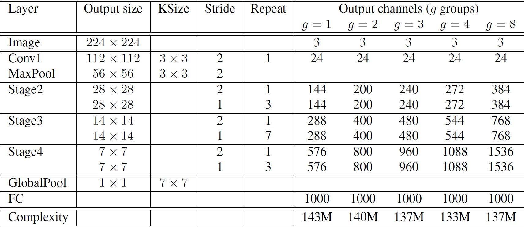
Image Courtesy: Official ShuffleNet paper
ShuffleNet V2
ShuffleNet V2 first postulates 4 guidelines for an efficient network architecture and presents an upgraded version of ShuffleNet that follows them. The 4 guidelines mentioned were:
-
Equal channel width minimizes memory access cost (MAC): It was observed that MAC is directly proportional to difference in channel width for the same FLOP's.
-
Excessive group convolution increases MAC: Experiments show that group size is directly proportional to MAC. Hence, increase in number of groups leads to more computation eventually hampering the speed.
-
Network fragmentation reduces degree of parallelism: Fragmentation is indirectly proportional to parallel computation.
-
Element-wise operations are non-negligible: Run-time decomposition charts show that simple element-wise operations are an overhead on speed.
Hence, an ideal network must have consistent channel width, reduce the number of group convolutions, element-wise operations and network fragmentation.
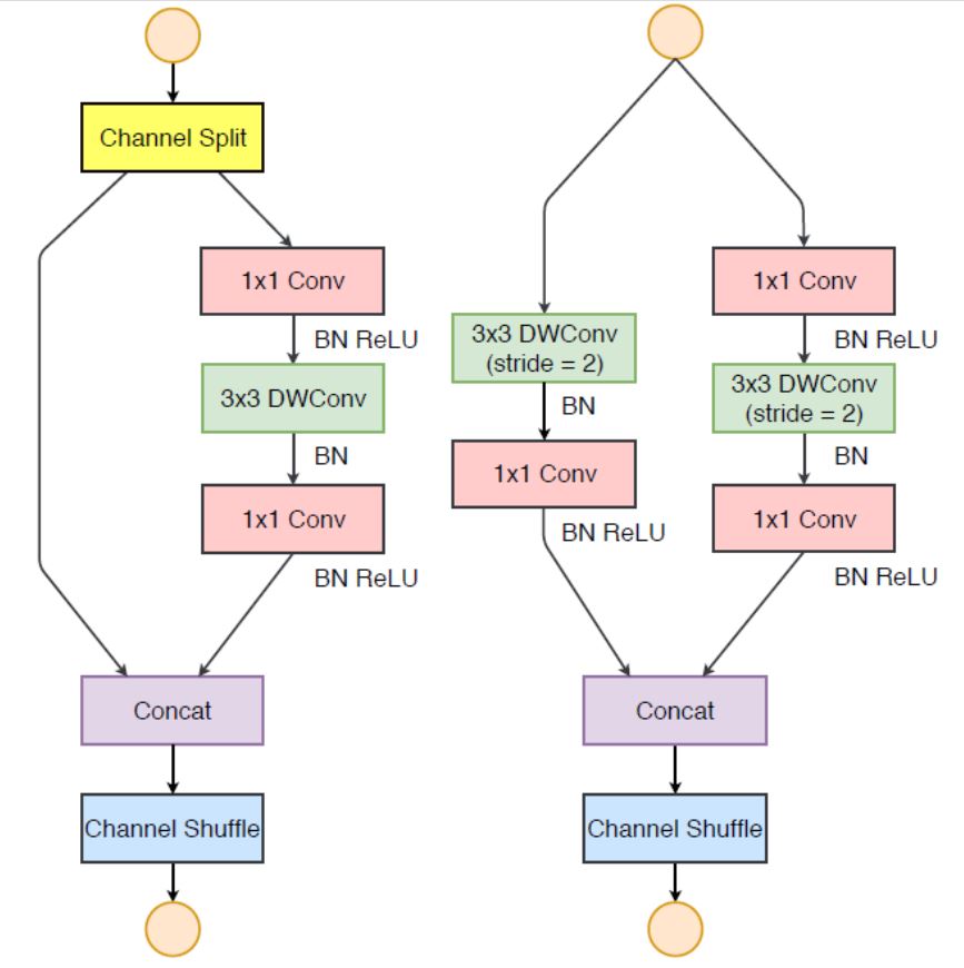
A typical ShuffleNet V2 looks as Figure 8. At the beginning of each unit, the input feature channels are divided into two branches. This is a simple Channel Split operation. Following third guideline, one branch remains as identity. The other branch consists of three convolutions with the same input and output channels to satisfy first guideline. The two 1×1 convolutions are no longer group-wise. This is partially to follow second guideline because the split operation already produces two groups. After convolution, the two branches are concatenated. So, the number of channels end up same. The same channel shuffle operation as in ShuffleNet V1 is then used to enable information communication between the two branches.
After the shuffling, the next unit begins. Note that the Add operation in ShuffleNet V1 no longer exists. Element-wise operations like ReLU and depth-wise convolutions exist only in one branch. Also, the three successive element-wise operations; Concat, Channel Shuffle and Channel Split, are merged into a single element-wise operation. These changes are beneficial according to fourth guideline.
One difference from ShuffleNet V1: An additional 1×1 convolution layer is added right before global averaged pooling to mix up features, which is absent in ShuffleNet V1.
ShuffleNet V2+
ShuffleNet V2+ varies from ShuffleNet V2 by adding Hard-Swish activation, Hard-Sigmoid activation and Squeeze and Excitation(SE) modules. Hard Swish activation and Hard- Sigmoid are based on slight variation and mix and match of RELU and sigmoid functions. SE modules improves channel interdependencies at almost no computational cost and hence are best suited for tiny devices. It is just a simple additional block that is added. This makes V2+ highly efficient incremental version of ShuffleNet V2.
ShuffleNetV2.Large
ShuffleNet V2-Large is deeper version of ShuffleNet V2 that consists of 140.7M tunable parameters. It is an extension of ShuffleNet V2 and hence works on following all guidelines by implementing Channel Split and Concat Operation with removal of grouped convolutions same its parent.
ShuffleNetV2.ExLarge
Similar to ShuffleNet V2-Large, the ShuffleNet V2- Extra Large is based on ShuffleNet V2. The only difference is the depth, which means it has repeated units of similar structure as its predecessor. The trainable parameters are 254.7M in number which is the double of ShuffleNet V2-Large and more than 110 times that of ShuffleNet V2.
Other similar Architectures?
The following CNN architectures have similar pattern of inter-mixing channel-level features and use grouped convolutions. I recommend you to check them out.
- ChannelNets: Compact and Efficient Convolutional Neural Networks via Channel-Wise Convolutions
- AddressNet: Shift-based Primitives for Efficient Convolutional Neural Networks
- CondenseNet: An Efficient DenseNet using Learned Group Convolutions
Parting Notes
The breakthrough CNN architecture for object classification in tiny mobile devices, ShuffleNet has been explained in depth in this article. Its newer and better version ShuffleNet V2 has also been elucidated. An introduction to the latest versions in the ShuffleNet family i.e. its large and extra large versions that support larger devices is also covered.
Coming up next in the series : How does ShuffleNet family compare with top architectures including VGG 16, MobileNet, GoogLeNet, SqueezeNet and AlexNet?
References
- To understand the working of CNN, refer this youtube video by Brandon Rohrer.
- To get an understanding of Grouped Convolution in depth, one can refer to this article by Yani Ioannou.
- Video contains depth explanation of Depth-wise convolution by Code Emporium.
- Pre-print of ShuffleNet research work by Xiangyu Zhang, Xinyu Zhou, Mengxiao Lin & Jian Sun.
- Pre-print of ShuffleNet V2 : Practical Guidelines for Efficient CNN Architecture Design by Ningning Ma, Xiangyu Zhang, Hai-Tao Zheng & Jian Sun1.
- Github Link of the whole ShuffleNet series.