In this article, we will understand why time series analysis is important and how it is done using different techniques like Spectral analysis amd different time series models like Auto-regressive (AR) model.

Table of contents

• Why is time series analysis important?
• Time series analysis methods
  • Spectral analysis
  • Wavelet analysis
  • Autocorrelation
  • Cross-correlation
• Time series models
  • Auto-regressive (AR) models
  • Moving average (MA) models
  • Integrated (I) model
  • ARMA
  • ARIMA
    
    

Why is time series analysis important?

Time series analysis can provide us with a better understanding of past events, thus enabling us to predict the future trends effectively. Prediction is made by discovering and analyzing underlying patterns in the time series data. Analysis of natural systems like climate, economic fluctuations and seismic activities can be extremely difficult without time series analysis. It is mainly used in the economic and business sectors to analyze the performance of stocks, predicting large downturns in business and many economic crises so that well-informed decisions can be made to avoid adverse effects. Time series analysis provides us with a way to predict the future and plays a key role in many major sectors.

Time series analysis methods

The methods used to analyze time series can be divided into two major categories:

• Time domain: Here, mathematical functions, signals and economical time series data are analyzed with respect to time. The time domain approach considers regression on past values of the time series. It includes the autocorrelation and cross-correlation methods.
• Frequency domain: Here, the mathematical functions and signals are analyzed with respect to frequency rather than time. The frequency domain approach considers regression on sinusoids. It includes spectral and wavelet analysis.
  
  

Spectral analysis

Often, the periodic behavior of a time series can be very complex. Spectral analysis allows us to discover underlying periodicities. This is widely used in oceanographic, atmospheric science, astronomy and various other fields. The main idea of spectral analysis is to decompose a stationary time series (x_t) into a combination of sines and cosines with unrelated and random coefficients as:

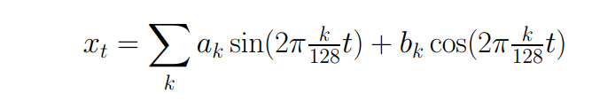
where,

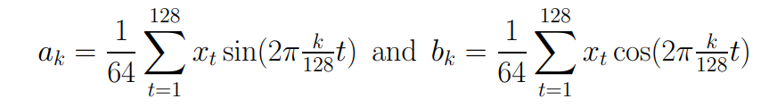
Let S_k = 0.5(a_k² + b_k²). This S_k over all k/128 frequencies is known as a spectrum. Spectrum breaks down the sample variance of time series into smaller pieces, each of which is associated with a particular frequency. We can get the approximate value of the spectral density by using a periodogram. It is the squared correlation between our time series and sine/cosine waves at the different frequencies spanned by the series.

Wavelet analysis

A wavelet is a mathematical function used in digital signal processing and image compression that is localized in time and frequency, generally with a zero mean. It tells us about variations in local averages. Wavelets are constructed by taking differences of scaling functions. The wavelet transform contains information on both the time location and frequency of a signal. Some typical properties of wavelets are:

• Orthogonality - Both wavelet transform matrix and wavelet functions can be
  orthogonal.
• Zero Mean (admissibility condition) - Forces wavelet functions to wiggle (oscillate between positive and negative).
• Compact Support - Efficient at representing localized data and functions.

Note that while these may be some typical properties, it is not required for wavelets to have these properties. Wavelets are analysis tools for time series and image analysis.

Autocorrelation

Similar to correlation, autocorrelation measures the linear relationship between a time series and lagged version of itself over subsequent time intervals. In simple terms, autocorrelation measures the relationship between a variable's present value and its past value that we have access to. The time interval between the two observations is referred to as lag. This method is used to discover underlying trends and patterns in the time series.

Mathematically, let the two terms y_t and y_t-k be separated by k time units, where k is the lag. Depending on the nature of data, this lag can be hours, days, months or years. If k=1, we are working with data points that are adjacent. The autocorrelation function for a time series is given by Corr(y_t , y_t-k) , k = 1,2,3.... This function is visualized using graphs to get a better understanding.

It is important to note that methods like regression modeling assume that there is no autocorrelation between residuals. Often this fact is ignored and people tend to assess if their model is a good fit using residuals. This may lead to misleading conclusions.

Cross-correlation

In the relationship between two time series x_t and y_t, the series y_t may be related to past lags of the x-series. The cross-correlation function is helpful for identifying lags of the x-variable that might be useful predictors of y_t. Simply put, cross-correlation tracks the movements of two variables relative to each other. It is used while measuring information from two different time series. Cross-correlation may also reveal any periodicities in the data.

For example, let us consider 3 variables A,B and C where A is the independent variable and B,C are dependent variables. Since B is dependent on A, they have a positive correlation and hence if the value of A increases, the value of B too increases. Similarly, since C is dependent on A, if the value of A increases, the value of C too increases. We can now say that the variables B and C are cross correlated as their behaviors are positively correlated as a result of each of their individual relationships to variable A.

Time series models

While performing time series analysis, we will be working with three core models. They are auto-regressive model, moving average model and integrated model.

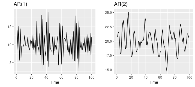
Auto-regressive (AR) models are simple linear regression models that predicts future performance based on past performance. It is used to represent a type of random process and uses lagged time variables as input. The equation for an AR model is:

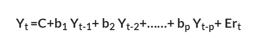
where;

• p is the past value
• Y_t is the function of different past values
• Er_t are the errors in time
• C is the intercept

Given below are two AR model simulated data.

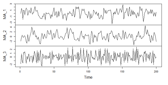
Moving average (MA) models are commonly used for modeling univariate time series. This model uses past forecast errors in a regression like model. The equation is:

where ε_t is the white noise. This a MA model of order q and is not really a regression as we do not observe the values of ε_t. Here, each value of y_t can be thought of as a weighted moving average of the past few forecast errors. Given below are three moving average models simulated from a dataset.

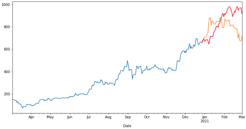
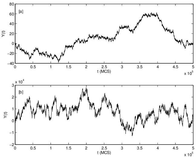
An Integrated (I) model is the one where all the data points are listed in time order. It uses the differencing of observation and makes the stationary data. Given below is an integrated time series model.

Other models used are ARMA which is a combination of auto-regressive and moving average models and ARIMA is a combination of all the three models. An example is given below for ARIMA model.