In this article, we will learn about a beginner-level approach to time series classification.

Table of Contents

• Introduction
• Dataset
• Installation/Setup
• Combining and Splitting the Data
• Feature Extraction
• Creating and Testing a Machine Learning Classifier
• Testing/Results
• Conclusion

Introduction

What is a time series?

A time series is a sequence of data points listed in chronological order. Usually, a time series is a sequence with measurements taken at equally spaced points in time.

Some common examples of time series data include stock prices and historical weather data. Time series is also common in patient health monitoring, such as in an electroencephalogram (EEG), which continuously measures neural activity, and an electrocardiogram (ECG), which monitors heart activity.

What is time series classification?

Time series classification is used to predict which category a time series belongs to. Based on several data points in a time series, time series classification is used to determine the class the entire time series belongs to.

Time Series Classification Approach

In this article, we will go over a beginner-level time series classification approach. Using the tsfresh Python library, we will first extract thousands of statistical features for each time series, including variance, skewness, standard deviation, and some more complex ones. We will then store these features in a tabular format, discard the unimportant features, and train a machine learning model on the resulting data.

Dataset

We will be walking through an application of time series classification used to predict the pattern of user movements in real-world office environments.

This problem involves determining whether or not an individual has moved between rooms based on time series of radio signal strength (RSS) between nodes of a Wireless Sensor Network (WSN).

The dataset was collected and made available by researchers from the University of Pisa in Italy. It is described in their paper An experimental characterization of reservoir computing in ambient assisted living applications.

Downloading the dataset

The dataset can be found in the UCI Machine Learning Repository using this link.

Dataset Structure

For our task, we will only be using the dataset directory. The dataset directory is organized as below:

dataset
    MovementAAL_RSS_1.csv
    MovementAAL_RSS_2.csv
    ...
    MovementAAL_target.csv

Each of the MovementAAL_RSS_{id} files represents a time series with measurements in chronological order and contains four columns representing the RSS measurements.

MovementAAL_target.csv contains the label for each of these time series. The target class 1 represents location changing movements, while -1 reprents location preserving movements.

Installation and Setup

Use the following pip commands to install the necessary libraries:

pip install pandas
pip install numpy
pip install scikit-learn

Import some of the main libraries and modules we need:

import os

import numpy as np
import pandas as pd

We will import more libraries and modules when we need them.

Combining and Splitting the Data

We will combine all the individual RSS data files into one dataframe and split the data into 80% training and 20% testing.

Let's first load the class labels:

data_path = '..' # the root dataset path, change if necessary

target_df = pd.read_csv(os.path.join(data_path, 'dataset', 'MovementAAL_target.csv')) # read the labels CSV file

These are the first few rows of target_df:

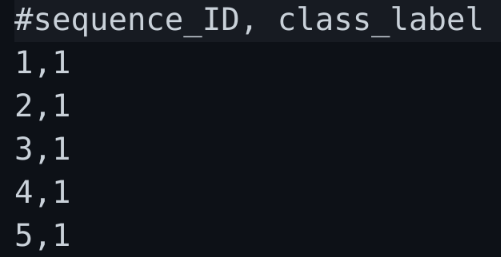
The column #sequence_ID represents the ID of each sequence, and we will later use this ID to refer to the sequence's corresponding time series CSV file.

Next, since there is a space between #sequence_ID and class_label, pandas reads the second column as " class_label", with an extra space at the beginning. We will remove this space so that the data will be easier to use later.

labels = target_df[' class_label']
labels.rename('class_label', inplace=True) # remove the leading whitespace

Next, we will create a list containing each sequence's ID.

sequence_ids = target_df['#sequence_ID']

Splitting Data

The code will be much simpler if we split the data before combining each of the individual sequences. By doing this, we will have an ID list of each of the training sequences as well as a separate testing ID list.

from sklearn.model_selection import train_test_split
train_ids, test_ids, train_labels, test_labels = train_test_split(sequence_ids, labels, test_size=0.2)

Now, we will create two dataframes, one for the training data and the other for the testing data.

X_train = pd.DataFrame()
X_test = pd.DataFrame()

Now, will loop through the training sequence IDs and the testing sequence IDs. For each of these sequence IDs, we will read the corresponding RSS time series data CSV file and add it to the main dataframe. We will also add a column for the sequence number and a step column which contains integers representing the time step in the sequence (e.g. whether it is the first or second measurement in the time series).

for i, sequence in enumerate(train_ids):
    df = pd.read_csv(os.path.join(data_path, 'dataset', f'MovementAAL_RSS_{sequence}.csv'))
    df.insert(0, 'sequence', i)
    df['step'] = np.arange(df.shape[0]) # creates a range of integers starting from 0 to the number of the measurements.
    X_train = pd.concat([X_train, df])

for i, sequence in enumerate(test_ids):
    df = pd.read_csv(os.path.join(data_path, 'dataset', f'MovementAAL_RSS_{sequence}.csv'))
    df.insert(0, 'sequence', i)
    df['step'] = np.arange(df.shape[0])
    X_test = pd.concat([X_test, df])

Feature Extraction

Now, we will use the tsfresh Python library to extract features.

The following code will generate a comprehensive feature set with over 3,000 features. The parameter column_id is the column that indicates which time series a measurement belongs to. The parameter column_sort is used to sort the measurements for each time series. However, this is not necessary for us since the dataset already contained measurements in chronological order. The code takes about 1-2 minutes to run.

from tsfresh import extract_features

extracted_features = extract_features(X_train, column_id='sequence', column_sort='step')

extracted_features now contains over 3000 columns. Now, we will impute all missing values and keep only the relevant features.

from tsfresh import select_features
from tsfresh.utilities.dataframe_functions import impute

impute(extracted_features)
train_labels = train_labels.reset_index() # reset the index 
features_filtered = select_features(extracted_features, train_labels['class_label'])

After this, we just have around 300 columns. This reduction will decrease model training time without losing any important information.

Now, let's extract features for the testing data and impute the missing values.

test_features =  extract_features(X_test, column_id='sequence', column_sort='step')
impute(test_features)

We will keep the same columns we kept in the training data.

test_features_filtered = test_features[features_filtered.columns]

Creating and Testing a Machine Learning Classifier

We will create a Random Forest classifier composed of 1000 decision trees.

from sklearn.ensemble import RandomForestClassifier
rf = RandomForestClassifier(n_estimators = 1000)
rf.fit(features_filtered, train_labels['class_label'])

Now, let's test the accuracy:

from sklearn.metrics import accuracy_score
print(accuracy_score(test_labels, rf.predict(test_features_filtered)))

0.9206349206349206

As shown above, our model performs with ~92% accuracy.

Conclusion

In this article, we learned a beginner-level time series classification method. Our final model ended up performing with over 92% accuracy. If you are interested in the results of other models and techniques applied on this dataset, take a look at my GitHub repository.

That's it for this article, and thank you for reading.

References:

• Bacciu, D., Barsocchi, P., Chessa, S., Gallicchio, C., & Micheli, A. (2013). An experimental characterization of reservoir computing in ambient assisted living applications. Neural Computing and Applications, 24(6), 1451–1464. https://doi.org/10.1007/s00521-013-1364-4
• Christ, M., Braun, N., Neuffer, J., & Kempa-Liehr, A. W. (2018). Time Series FeatuRe Extraction on basis of Scalable Hypothesis tests (tsfresh – A Python package). Neurocomputing, 307, 72–77. https://doi.org/10.1016/j.neucom.2018.03.067