In this article, we have explained the idea of Adjacency Matrix which is good Graph Representation. We have presented it for different cases like Weighted, undirected graph along with implementation and comparison with Adjacency List.

Table of contents:

• Introduction to graph representation
• Adjacency Matrices explained
• Case 1: Unweighted, undirected graph
• Case 2: Unweighted, directed graph
• Case 3: Weighted, undirected graph
• Case 4: Weighted and directed graph
• C++ Implementation
• Comparison: Adjacency Matrix vs Adjacency List

Let us get started with Adjacency Matrix.

Introduction to graph representation

Graphs are defined as a structure which shows the relationships between a set of objects. These graphs contain vertices (also known as nodes), which are the individual points on a graph, and edges (also known as arcs), representing the connections between the verticies. Graphs can be weighted when there are "costs" along each edge and also directed, meaning that traversal can only happen in a particular direction.

Adjacency Matrices explained

Let's say we have a graph with the number of vertices (n) and a set number of edges (e). From this, we can deduce that (i,j) is an edge starting at i and ending at j, if i and j both represent vertices. An adjacency matrix is a way of representing the relationships of these vertices in a 2D array. For unweighted graphs, if there is a connection between vertex i and j, then the value of the cell [i,j] will equal 1, if there is not a connection, it will equal 0. When graphs become weighted, the value of 1 is replaced with the "cost" of the edge, and the connectionless cells can be changed to the infinity symbol.

Case 1: Unweighted, undirected graph

Take for example this graph:

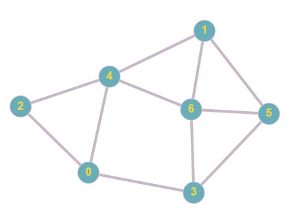
Currently there are no directions or weights involved, there are 7 total nodes, 0-6. We can represent this in an adjacency matrix using the steps above.

Explanation:

In this adjacency matrix, 1 represents a connection and 0 represents no connection. In this case we take a particular node, check which other nodes it is connected to, and plot in the matrix a binary value based on this. In undirected graphs, the matrix will always be symmetrical since if two nodes have a connection, they are connected in both ways, this changes in the case direction is involved, as will be demonstrated in later examples

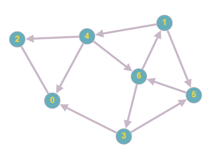
Case 2: Unweighted, directed graph

We now can add directions to the previous graph, then see how that affects the matrix

The adjacency matrix for the new graph would be:

Explanation:

As you can see, the graph now contains directions. This will alter the matrix since nodes are connected only in a specific direction. For example, in row 1, there now contains only 2 rather than 3 since node 1 is still connected to node 4 and 5, however there is no longer a connection to 6 as there is a different edge direction. We can see that this is mirrored throughout the new matrix, with connections only being present when the direction is correct.

Case 3: Weighted, undirected graph

The next stage in our adjacency matrix journey is involving weights. This can be implemented through similar methods to a standard matrix, however instead of the values of each cell being binary, we replace it with the weight of each edge. If there is not a connection, we can represent this by using the infinity symbol.

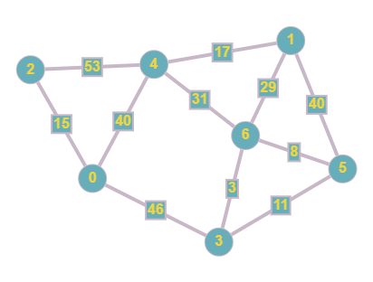
As you can see we now have added weights to the edges in our graph, this means that during traversal, there will be a cost for travelling across a particular edge. We can then plot this in our matrix by following the aforementioned steps.

Explanation:

This matrix is similar to the original one that we created, however the 0 values have now been plotted as the infinity symbol (cannot use 0 since that would imply a connection with a cost of 0) and the 1 values are replaced with the cost of each edge.

Case 4: Weighted and directed graph

Our final graph in this explanation involves everything we have covered so far, combining weights and directions.

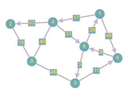
The same weights and directions from the previous graphs have been used however we now have implemented them on the same graph. This means that each edge has a particular direction that needs to be followed when traversing in addition to having a "cost", which needs to be taken into account when conducting things like a shortest path search.

Explanation:

This is our final adjacency matrix, we can see that the connections are in the same cells as in Case 2 however using the same values as in Case 3. This is because the graph is both weighted and directed. This means that the matrix cannot be symmetrical since nodes are only connected in a certain direction, the infinity symbol must be used instead of 0 since we have to show that there is no connection present instead of a connection with a cost of 0, and the costs must be used as the values instead of 1 to denote the weight of each edge.

C++ Implementation

Here is an implementation for the adjacency matrix from Case 1 in C++

#include <iostream>
using namespace std;

class Graph {
   private:
  bool** adjMatrix;
  int numVtx;

   public:
  
  Graph(int numVtx) {
    this->numVtx = numVtx;
    adjMatrix = new bool*[numVtx];
    for (int i = 0; i < numVtx; i++) {
      adjMatrix[i] = new bool[numVtx];
      for (int j = 0; j < numVtx; j++)
        adjMatrix[i][j] = false;
    }
  }
  
  void addEdge(int i, int j) {
    adjMatrix[i][j] = true;
    adjMatrix[j][i] = true;
  }

  void deleteEdge(int i, int j) {
    adjMatrix[i][j] = false;
    adjMatrix[j][i] = false;
  }

  void toString() {
    for (int i = 0; i < numVtx; i++) {
      cout << i << " : ";
      for (int j = 0; j < numVtx; j++)
        cout << adjMatrix[i][j] << " ";
      cout << "\n";
    }
  }

  ~Graph() {
    for (int i = 0; i < numVtx; i++)
      delete[] adjMatrix[i];
    delete[] adjMatrix;
  }
};

int main() {
  Graph g(7);

  g.addEdge(0, 2);
  g.addEdge(0, 3);
  g.addEdge(0, 4);
  g.addEdge(1, 4);
  g.addEdge(1, 5);
  g.addEdge(1, 6);
  g.addEdge(2, 0);
  g.addEdge(2, 4);
  g.addEdge(3, 0);
  g.addEdge(3, 5);
  g.addEdge(3, 6);
  g.addEdge(4, 0);
  g.addEdge(4, 1);
  g.addEdge(4, 2);
  g.addEdge(4, 6);
  g.addEdge(5, 1);
  g.addEdge(5, 3);
  g.addEdge(5, 6);
  g.addEdge(6, 1);
  g.addEdge(6, 3);
  g.addEdge(6, 4);
  g.addEdge(6, 5);

  g.toString();
}

Comparison: Adjacency Matrix vs Adjacency List

So far, we have discussed the use of adjacency matrices in the representation of graphs, an alternative method would be the implementation of an adjacency list. An adjacency list is similar to an adjacency matrix in the fact that it is a way of representing a graph, however it uses linked lists to store the connections between nodes. Each element in the array is a linked list containing all connected vertices.

For example here is an adjacency list for the graph in Case 2:

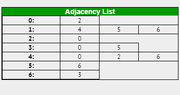
If the graph was weighted, the same principles apply however along with the vertex you would also include the cost of travel in each element

Time/Space Complexities

Adjacency Matrix:

Space complexity: O(N * N)
Time complexity for checking if there is an edge between 2 nodes: O(1)
Time complexity for finding all edges from a particular node: O(N)

Adjacency List:

Space complexity: O(N+M)
Time complexity for checking if there is an edge between 2 nodes: O(degree of node)
Time complexity for finding all edges from a particular node: O(degree of node)

Applications

As you can see above, the differing complexities of each representation mean they are best suited to different purposes. Since the space complexity of adjacency lists is more efficient than the matrix, it is best suited for sparsely populated graphs (ones with a small edge count) where as the matrix is best for dense graphs (ones with a large edge count).

Adjacency Matrix:

A well known algorithm where matrices are best used is the All-Pairs Shortest Path algorithm, since this pathfinding requires information about all possible edges. As the data in an adjacency matrix is held in individual cells, this means indexing is very efficient, making it the better choice to implement in this algorithm.

Adjacency List:

Adjacency lists however are the preferred option in the majority of use cases, unless the algorithm is dependant on a matrix, it is for many common pathfinding and searching algorithms such as Dijkstra's and Breadth/Depth First Search due to it being more space efficient.

With this article at OpenGenus, you must have the complete idea of Adjacency Matrix.