In this article, we will be comparing the performance of different data preprocessing techniques (specifically, different ways of handling missing values and categorical variables) and machine learning models applied to a tabular dataset. We will go over all the steps separately and them combine them in the end.

Table of Contents

• Introduction
• Installation and Setup
• Dataset Loading and Preparation
• Handling Missing Values
• Handling Categorical Variables
• Different Machine Learning Models
• Testing, Results, and Interpretation of Results
• Conclusion

Introduction

There are several steps involved in machine learning, including various preprocessing steps and creating/training a model.

There are multiple methods for each step of the machine learning workflow. We will be going over different methods for handling missing values and categorical variables, and we will also be going over different machine learning models.

We will first go over an explanation of different preprocessing techniques and machine learning models. Then, we will implement and compare them.

Handling Missing Values

Having missing values is a common problem in real-world datasets. A missing value is defined as data that is not present for some variable(s) in a dataset.

The dataset we will be using (more information about it later) contains missing values. The screenshot below shows two instances of missing values:

We'll be going over two techniques to handle missing values:

• Removing columns with missing values
• Imputation: Attempts to fill in missing values of a feature by using the mean of the column it is a numerical feature or by using the most frequent class if it is a categorical feature.

Handling Categorical Variables

Datasets contain categorical variables (variables that take one of a limited number of possible values) that are not represented by integers. For example, the dataset we will be using contains a column titled 'Sex', which is an example of a categorical variable.

Most machine learning models in Python will throw an error if we try to input categorical variables without preprocessing them first, so handling categorical variables is an essential step in machine learning.

We will look at three approaches for handling categorical variables:

• Removing categorical variables
• Ordinal encoding: assigns a unique number to each possible value. Example:
  
• One-hot encoding: creates new columns that indicate the presence or absence of each possible value in the original data. Example:
  

Different Machine Learning Models

There are a lot of different machine learning models that can be used for various types of problems. We'll be going over three different models:

• Support Vector Machine (SVM): Support Vector Machine (SVM) is a linear model for classification and regression problems that creates a line or a hyperplane that best separates the data into classes. The SVM tries to find the optimal hyperplane by finding the points closest to a line (called support vectors) and calculating the Euclidean distance between the line and the support vectors, which is called the margin, and the goal of the SVM is to maximize this margin. In other words, the SVM tries to make a boundary in such a way that the separation between different classes is as wide as possible.
  

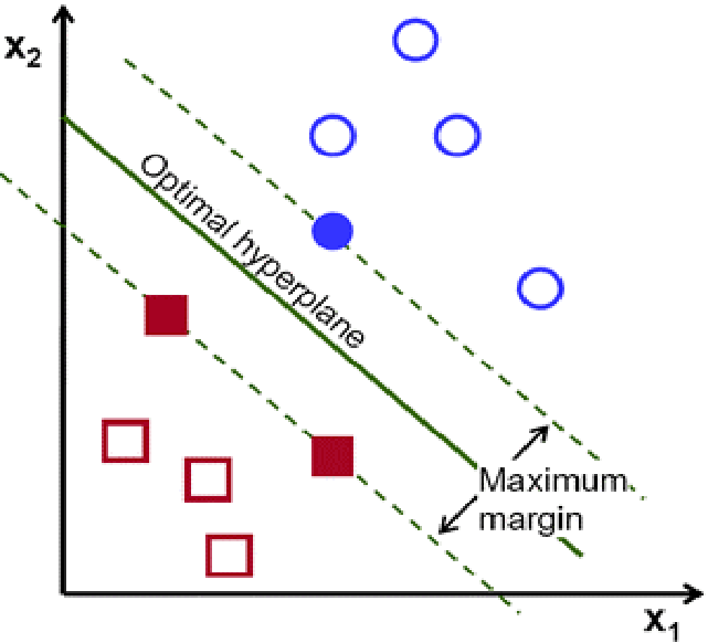
Above- Optimal Hyperplane and Margin of SVM (Fidan et al., 2020) This picture shows an optimal hyperplane that maximizes the margin (distance between the support vectors and the hyperplane)

• Logistic Regression: Logistic Regression is a supervised machine learning algorithm used to model the probability of a certain class or event. It is used when the data is linearly separable, usually in binary classification tasks. At the core of this algorithm is the logistic function (also called the sigmoid function), which can take any real number and map it into a value between 0 (excluded) and 1 (excluded). For this reason, the predicted y value of logistic regression is between 0 and 1, as opposed to linear regression, where the predicted y value can exceed this range.

• Random Forest: The Random forest algorithm consists of a large number of individual decision trees that operate as an ensemble. When predicting on a sample, each individual tree outputs a class and the class with the most “votes” is outputted as the prediction of the Random Forest. An advantage of Random Forest is that it is a non-black-box model, meaning that it can explain the steps it took to predict a particular outcome.

Installation and Setup

For this article, we will need the following libraries:

• Pandas
• NumPy
• Scikit-Learn
• XGBoost

Install the above libraries using pip:

pip install pandas
pip install numpy
pip install scikit-learn
pip install xgboost

Import the necessary libraries:

from warnings import filterwarnings

import numpy as np
import pandas as pd
from sklearn import svm
from sklearn.linear_model import LogisticRegression
from sklearn.ensemble import RandomForestClassifier
from sklearn.impute import SimpleImputer
from sklearn.metrics import accuracy_score
from sklearn.model_selection import train_test_split
from sklearn.preprocessing import OneHotEncoder, OrdinalEncoder
from xgboost import XGBClassifier

Dataset Loading and Preparation

For this article, we will be using the dataset from the Titanic-Machine Learning from Disaster Kaggle competition. It can be found using this link. We will be using the file "train.csv".

The goal is to determine whether or not a passenger of the Titanic would have survived given some information about them.

Reading the data

Load the data using pd.read_csv.

df = pd.read_csv("train.csv")

Let's view the first few rows of the dataset:

df.head()

Let's split df into X, which stores the features, and y, which stores the labels (the "survived" column). We won't be using "PassengerId" and "Name" to train our models, so we'll drop those columns as well.

y = df["Survived"]
X = df.drop(["Survived", "PassengerId", "Name"], axis=1) #drops all the columns we don't need in X

Splitting the data

We will split the dataset into 80% training and 20% validation. The models we train will be evaluated on the validation data.

X_train, X_valid, y_train, y_valid = train_test_split(X, y, train_size=0.8, test_size=0.2, random_state=0)

Handling Missing Values

To determine which columns in the dataset have missing values, we can run the following code:

cols_with_missing = [col for col in X_train.columns if X_train[col].isnull().any()]
print(cols_with_missing)

['Age', 'Cabin', 'Embarked']

As we can see, the columns "Age", "Cabin", and "Embarked" contain missing values.

There are multiple ways we can handle missing values, and we will go over two of them: removing columns with missing values, and using imputation.

Option 1 : Remove Missing Values

The easiest and simplest way to deal with missing values is to simply remove columns with missing values.

cols_with_missing = [col for col in X_train.columns if X_train[col].isnull().any()]
reduced_X_train = X_train.drop(cols_with_missing, axis=1)
reduced_X_valid = X_valid.drop(cols_with_missing, axis=1)

This could, however, possibly remove some important information.

Option 2 : Imputation

We can fill in missing values based on the mean for numerical features and the most frequent class for categorical features. We do this by creating two SimpleImputer objects, one with strategy "mean", used for the numerical columns, and the other with strategy "most_frequent", used for the categorical data.

# create a list of numerical columns
numerical_cols = X_train.select_dtypes(include=np.number).columns.tolist()

# create a list of categorical columns
s = (X_train.dtypes == 'object')
categorical_cols = list(s[s].index)

# create a copy of the original data so that none of the original data is changed
imputed_X_train = X_train.copy()
imputed_X_valid = X_valid.copy()

# create two imputers - one for the numerical columns, and the other for the categorical columns
numerical_imputer = SimpleImputer(strategy="mean")
categorical_imputer = SimpleImputer(strategy="most_frequent")

# use the imputer and update the training data
imputed_X_train[numerical_cols] = numerical_imputer.fit_transform(imputed_X_train[numerical_cols])
imputed_X_train[categorical_cols] = categorical_imputer.fit_transform(imputed_X_train[categorical_cols])

# use the imputer and update the validation data
imputed_X_valid[numerical_cols] = numerical_imputer.transform(imputed_X_valid[numerical_cols])
imputed_X_valid[categorical_cols] = categorical_imputer.transform(imputed_X_valid[categorical_cols])

Handling Categorical Variables

Some columns of the dataset are categorical variables (variables that take one of a limited number of possible values) and are not represented by integers.

To determine which features are categorical, we check the data type, or the dtype. In this dataset, the columns with text indicate categorical variables.

# Get list of categorical variables
s = (imputed_X_train.dtypes == 'object')
categorical_cols = list(s[s].index)

print("Categorical variables:")
print(categorical_cols)

Categorical variables:
['Sex', 'Ticket', 'Cabin', 'Embarked']

Let's inspect these categorical variables and take a look at the number of unique classes.

for feature in categorical_cols:
    print(f"{feature}: {len(imputed_X_train[feature].unique())}")

Sex: 2
Ticket: 569
Cabin: 127
Embarked: 3

We can see that columns "Ticket" and "Cabin" have many distinct values. For simplicity, we won't consider those columns.

# delete the "Ticket" and "Cabin" columns from both the training and validation data
imputed_X_train.drop(["Ticket", "Cabin"], axis=1, inplace=True)
imputed_X_valid.drop(["Ticket", "Cabin"], axis=1, inplace=True)
reduced_X_train.drop("Ticket", axis=1, inplace=True) # cabin was already dropped when missing values were dropped
reduced_X_valid.drop("Ticket", axis=1, inplace=True) # cabin was already dropped when missing values were dropped

Note: inplace=True directly updates the dataframe instead of returning a copy.

There are various methods for handling categorical features. We will look at three of them: dropping categorical features, ordinal encoding, and one-hot encoding.

For each of the different techniques, we will create functions so that they can easily be used when we are testing the final models.

Dropping categorical features

The easiest way to deal with categorical features is to drop them. This approach only works well if the columns do not contain useful information.

def drop_categorical_variables(train_df, valid_df):
    drop_train = train_df.select_dtypes(exclude=['object'])
    drop_valid = valid_df.select_dtypes(exclude=['object'])
    return drop_train, drop_valid

drop_X_train, drop_X_valid = drop_categorical_variables(imputed_X_train, imputed_X_valid)

The code above creates two new dataframes: drop_X_train and drop_X_valid. These two dataframes exclude all the columns with a type of object.

We can confirm that the categorical variables have been removed by outputting a list of columns drop_X_train contains.

print(list(drop_X_train.columns))

['Pclass', 'Age', 'SibSp', 'Parch', 'Fare']

Ordinal Encoding

Ordinal encoding assigns a different integer to each unique value.

For example, let's take a look at the different values of the "Embarked" column:

print(list(imputed_X_train["Embarked"].unique()))

['C', 'S', 'Q']

Let's encode each of the categorical variables:

def ordinal_encode(train_df, val_df):
    s = (train_df.dtypes == 'object')
    categorical_cols = list(s[s].index)

    # Apply ordinal encoder to each column with categorical data
    ordinal_encoded_X_train = train_df.copy()
    ordinal_encoded_X_valid = val_df.copy()

    ordinal_encoder = OrdinalEncoder()
    ordinal_encoded_X_train[categorical_cols] = ordinal_encoder.fit_transform(train_df[categorical_cols])
    ordinal_encoded_X_valid[categorical_cols] = ordinal_encoder.transform(val_df[categorical_cols])
    
    return ordinal_encoded_X_train, ordinal_encoded_X_valid

ordinal_encoded_X_train, ordinal_encoded_X_valid = ordinal_encode(imputed_X_train, imputed_X_valid)

Now, let's see how the values of the "Embarked" column changed.

print(list(ordinal_encoded_X_train["Embarked"].unique()))

[0.0, 2.0, 1.0]

One-hot encoding

One-hot encoding generates new columns that indicate the presence or absence of each possible value in the original data.

For example, when one-hot encoding is applied to the "Embarked" column, it would generate columns "C", "S", and "Q". Each of these columns would contain either 1 or 0, where 1 represents that the original data contained that value.

def one_hot_encode(train_df, validation_df):
    s = (train_df.dtypes == 'object')
    categorical_cols = list(s[s].index)

    # handle_unknown='ignore' helps avoid errors when the validation data contains classes that are not in the training data
    # sparse = false makes sure that it returns a numpy array instead of a sparse matrix
    encoder = OneHotEncoder(handle_unknown='ignore', sparse=False)

    # create new dataframes for the one-hot encoded features
    OH_cols_train = pd.DataFrame(encoder.fit_transform(train_df[categorical_cols]))
    OH_cols_valid = pd.DataFrame(encoder.transform(validation_df[categorical_cols]))

    # One-hot encoding removed the index, so we put it back here. 
    # This is used for combining the one-hot encoded columns with the numerical columns, otherwise alignment issues arise
    OH_cols_train.index = train_df.index
    OH_cols_valid.index = validation_df.index
    
    # fix the column names
    OH_cols_train.columns = encoder.get_feature_names_out()
    OH_cols_valid.columns = encoder.get_feature_names_out()
    
    # remove the original categorical columns
    num_X_train = train_df.drop(categorical_cols, axis=1)
    num_X_valid = validation_df.drop(categorical_cols, axis=1)

    # combine the encoded features to the numerical features
    OH_X_train = pd.concat([num_X_train, OH_cols_train], axis=1)
    OH_X_valid = pd.concat([num_X_valid, OH_cols_valid], axis=1)
    
    return OH_X_train, OH_X_valid

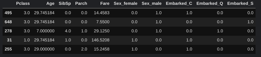
OH_X_train, OH_X_valid = one_hot_encode(imputed_X_train, imputed_X_valid)
OH_X_valid.head()

Different Machine Learning Models

We will be training and evaluating three different models - Support Vector Machine (SVM), Logistic Regression, and Random Forest.

In the following examples, we'll be training on the one-hot encoded data.

Support Vector Machine (SVM)

Support Vector Machine is a supervised machine learning algorithm that separates the data into classes using a hyperplane or line.

The code below creates and trains a Support Vector Machine model:

svm_clf = svm.LinearSVC()
svm_clf.fit(OH_X_train, y_train)

Logistic Regression

Logistic regression predicts the probability of the output class by fitting data to a logit function.

lr=LogisticRegression()
lr.fit(OH_X_train, y_train)

Random Forest

Random Forest is an ensemble model made up of several Decision Trees.

clf = RandomForestClassifier()
clf.fit(OH_X_train, y_train)

Depending on the categorical variable encoding techniques used, we would pass different dataframes into fit.

Testing, Results, and Interpretation of Results

We will create a list of all the training and validation dataframes using which we will train the models. First, we'll create a list of the dataframes with handled missing values. For each dataframe, there is a description along with the training and validation data, represented by a dict.

# make sure none of the dataframes contains the "Ticket" or "Cabin" columns - if they do, uncomment the code below
# imputed_X_train.drop(["Ticket", "Cabin"], axis=1, inplace=True)
# imputed_X_valid.drop(["Ticket", "Cabin"], axis=1, inplace=True)
# reduced_X_train.drop(["Ticket", "Cabin"], axis=1, inplace=True)
# reduced_X_valid.drop(["Ticket", "Cabin"], axis=1, inplace=True)

missing_values_handled_dfs = [
    {
        "description" : "Dropped Missing Values", 
        "train" : reduced_X_train, 
        "validation" : reduced_X_valid
    },
    {
        "description" : "Imputed", 
        "train" : imputed_X_train, 
        "validation" : imputed_X_valid
    }
]

Next, we will use apply different categorical variable handling techniques and create a list of all possible pairs of dataframes (training and validation). In other words, for each missing value handling technique, there are three different pairs of dataframes, each representing one of the three categorical variable handling techniques used. This way, we end up with 6 pairs of dataframes.

dfs_to_be_used = [] #list of dictionaries - each dict will contain a description, the training dataframe, and the validation dataframe

for df_dict in missing_values_handled_dfs:
    train_df = df_dict["train"]
    validation_df = df_dict["validation"]
    description = df_dict["description"]
    
    # drop categorical features
    drop_X_train, drop_X_valid = drop_categorical_variables(train_df, validation_df)
    dfs_to_be_used.append({
        "description" : description + ", dropped categorical features",
        "train" : drop_X_train,
        "validation" : drop_X_valid
    })
    
    # ordinal encoding
    ordinal_encoded_X_train, ordinal_encoded_X_valid = ordinal_encode(train_df, validation_df)
    dfs_to_be_used.append({
        "description" : description + ", ordinal encoding ",
        "train" : ordinal_encoded_X_train, 
        "validation" : ordinal_encoded_X_valid
    })
    
    #one-hot encoding
    OH_X_train, OH_X_valid = one_hot_encode(train_df, validation_df)
    dfs_to_be_used.append({
        "description" : description + ", one-hot encoding ",
        "train" : OH_X_train, 
        "validation" : OH_X_valid
    })

Next, we'll test all the different models on each of these 6 dataframes and record the results.

When training some models, there are sometimes warnings that are outputted. We can disable these warnings by running the following code:

filterwarnings('ignore')

This will make it easier to read the results.

The following code outputs the results of each model for each of the different dataframes. y_train and y_valid, which are used below, were created towards the beginning of this article when we split the data into 80% training and 20% validation.

for df in dfs_to_be_used:
    print(df["description"] + ":")
    
    svm_clf = svm.LinearSVC()
    svm_clf.fit(df["train"], y_train)
    
    print("\t" + "SVM: " + str(accuracy_score(y_valid, svm_clf.predict(df["validation"]))))
    
    lr=LogisticRegression()
    lr.fit(df["train"], y_train)
    
    print("\t" + "Logistic Regression: " + str(accuracy_score(y_valid, lr.predict(df["validation"]))))
    
    rf = RandomForestClassifier()
    rf.fit(df["train"], y_train)
    
    print("\t" + "Random Forest: " + str(accuracy_score(y_valid, rf.predict(df["validation"]))))

Dropped Missing Values, dropped categorical features:
	SVM: 0.7262569832402235
	Logistic Regression: 0.7150837988826816
	Random Forest: 0.7150837988826816
Dropped Missing Values, ordinal encoding :
	SVM: 0.776536312849162
	Logistic Regression: 0.7988826815642458
	Random Forest: 0.8324022346368715
Dropped Missing Values, one-hot encoding :
	SVM: 0.6759776536312849
	Logistic Regression: 0.7988826815642458
	Random Forest: 0.8379888268156425
Imputed, dropped categorical features:
	SVM: 0.6983240223463687
	Logistic Regression: 0.7374301675977654
	Random Forest: 0.6927374301675978
Imputed, ordinal encoding :
	SVM: 0.664804469273743
	Logistic Regression: 0.7988826815642458
	Random Forest: 0.8324022346368715
Imputed, one-hot encoding :
	SVM: 0.8100558659217877
	Logistic Regression: 0.8044692737430168
	Random Forest: 0.8435754189944135

As we can see above, the highest performing model in this case was the Random Forest model that was trained on the imputed and one-hot encoded data.

Models tended to perform better with encoded categorical features over removed categorical features. One-hot encoding versus ordinal encoding didn't seem to make much of a difference for this experiment, although one-hot encoding usually performs better in most situations. Also, imputation didn't make much of a difference either, but imputation is generally a better choice than removing missing values.

Conclusion

In this article, we saw how different machine learning models and preprocessing techniques compare to each other in terms of performance. This article outlined some of the most common ones, but there are several other preprocessing techniques and models that could be used to achieve different results.

That's it for this article, and thanks for reading!