
Get this book -> Problems on Array: For Interviews and Competitive Programming
In this article, we have explored the concept of Markov chain along with their definition, applications, and operational details. We have covered how Markov Chain is used in the field of Deep Learning/ Neural Network.
Table of contents:
- Introduction
- Basic Concept
- Markov chain types
- Markov Chains Properties
- Example
- Applications
6.1. Markov Chain applications in Neural Networks - Markov chain neural network
- Conclusion
Introduction
Markov chains are mathematical structures that jump from one "state" (a circumstance or collection of values) to another. They are named after Andrey Markov. For instance, if you created a Markov chain model of how a washing machine behaves, you might include the states "idle," "operating/washing," and "operating/drying" which, along with other behaviors, could create a "state space": a list of all possible states. In addition, on top of the state space, a Markov chain tells you the probability of hopping, or "transitioning," from one state to any other state—-e.g., the chance that a washing machine currently "operating/washing will be "idle" in the next 3 minutes without "operating/drying".
Basic Concept
A Markov chain is a type of stochastic process; however, unlike other types of stochastic processes, a Markov chain must be "memory-less" in order to function properly. That is to say, the actions that will take place in the future are not dependent on the sequence of events that brought about the current state. This is known as the Markov property. There are many common examples of stochastic properties that do not satisfy the Markov property, despite the fact that the theory of Markov chains is important for the very reason that so many "everyday" processes satisfy the Markov property. However, the theory of Markov chains is important.
Markov chain types
There are two kinds of Markov chains. These are discrete-time Markov chains and continuous-time Markov chains.
-
Markov chains known as continuous-time Markov chains (CTMC) have state transitions that happen at random times as opposed to discrete intervals of time. Instead of using probabilities, rate functions define the transition probabilities. For instance, a CTMC's state could stand in for the volume of customers entering and leaving a store at any given moment, and changes in state could be interpreted as customer movement. The CTMC model can be used to calculate the probability of a system being in a specific state (for example, the probability that there are a certain number of customers in the store).
-
Discrete-time Markov chains, also known as DTMCs, are a special type of Markov chain in which the transitions between states take place at regular intervals of discrete time. A transition matrix defines the transition probabilities. For instance, a DTMC's state (such as sunny, cloudy, or rainy) could stand in for the weather on a specific day, and transitions between states could stand in for the weather's shift from one day to the next. The DTMC model can calculate the probability of a system being in a specific state (for example, the probability of it being sunny on a specific day).
Markov Chains Properties
In what follows, we will discuss a few of the Markov Chain's more typical features, characteristics, and properties.
-
Irreducibility
If there is a transition between any two states in a given time step, the Markov chain is said to be irreducible. -
Periodicity and Absorbing States
When we talk about a state being absorbing, we mean that once we get there, we can't get out of it anymore. To put it another way, there is an absolutely certain chance that it will revert to its previous state. -
Transient and Recurrent States
If there is a chance that the chain won't ever return to a particular state again after entering it, that state is said to be** transient**.
A recurrent state is one that does not change very frequently. As a result, the probability of entering a specific state is 1, and the chain will undoubtedly return to that state indefinitely.
Example
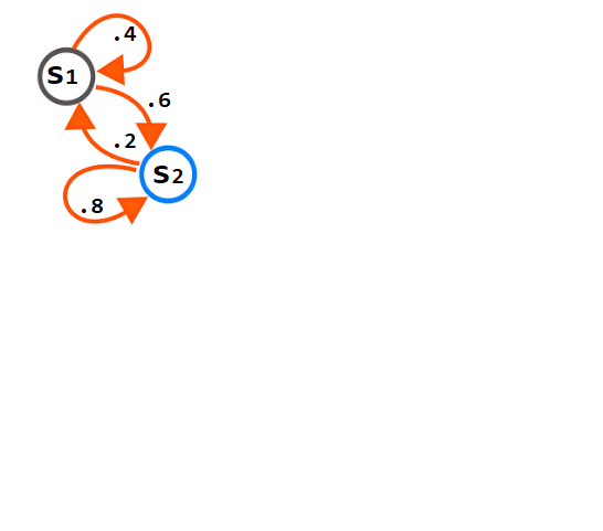
Fig1. Simple Markov Model
The graphical representation below indicates a Markov process with two states, denoted here as S1 and S2. In this case, the arrows started at the present state and point to the future state; the number that is connected with the arrows reflects the likelihood that the Markov process will change from one state to another state.
For instance, if the Markov process is currently in state S1, then the likelihood that it will transition to state S2 is 0.6, whereas the probability that it would continue to exist in the same state is 0.4. Similarly, for every process in state S2, the probability of changing to S1 is 0.2, whereas the likelihood of remaining in the same state is.8.
Implementing the previous Markov process uisng Python code
import scipy.linalg
import numpy as np

state = ["A", "E"]

MyMatrix = np.array([[0.6, 0.4], [0.7, 0.3]])

n = 20
StartingState = 0
CurrentState = StartingState

print(state[CurrentState], "--->", end=" ")

while n-1:
  random.choice()
    CurrentState = np.random.choice([0, 1], p=MyMatrix[CurrentState])
    print(state[CurrentState], "--->", end=" ")
    n -= 1
print("stop")

MyValues, left = scipy.linalg.eig(MyMatrix, right=False, left=True)

print("left eigen vectors = \n", left, "\n")
print("eigen values = \n", MyValues)

pi = left[:, 0]
pi_normalized = [(x/np.sum(pi)).real for x in pi]
pi_normalized
Here, we note the following:
- The necessary librares have been impoterd first, which are scipy and numpy.
- The states (S1 & S2) have been declared and their transitions value have been assigned to a matrix called transition matix (A Markov transition matrix is a square matrix that describes the probabilities of changing states in a dynamic system.)
3.On our Markov chain, we simulate a random walk with 20 steps. We just start with an arbitrary state and go through our Markov chain when we random walk.Then, using a random choice( ), to choose the next state.
4.Last but not least, we should determine the stationary distribution of our by locating the left eigen vectors.
5 Note: that since Pi is a probability distribution, the total of all of the probabilities ought to equal 1. To extract that from the negative values presented earlier, all we need to do is normalize the data.
Markov Chains Applications
Markov chains are useful statistical models for a wide variety of real-world phenomena, including the analysis of cruise control systems in motor vehicles, lineups or lines of clients arriving at an airport, rates of currency exchange, and the dynamics of animal populations. In addition, Markov chains are used in speech recognition, music production, and search engine algorithms.
Markov Chain applications in Neural Networks
An artificial neural network, also known as an ANN, is a specific type of machine learning model that was developed to simulate the structure and performance of the human brain. They are composed of layers of connected "neurons" that process information and generate predictions in response to input. Predictive modeling, image recognition, and natural language processing are just a few of the many tasks that ANNs are used for.
One application of Markov chains in Neural Networks that many of us use on a daily basis is the predictive text feature on mobile devices. You may have discovered that predictive text becomes "smarter" the more you use your phone, eventually suggesting words that are unique to you and your environment. This is because the software is gradually building a Markov chain based on your typing patterns and computes the likelihood of the next word you'll type based on what you've already typed.
Classifiers are another application for Markov Chains. A classifier is a specific kind of machine learning algorithm that is used to assign a class label to the data input it receives. The labeling of an image with terms like "car," "truck," or "person" is an example of an image recognition classifier.
Markov chain neural network
In this section we are going to review The fundamental concept behind a propsed non-deterministic MC neural network,by "Maren Awiszus, et al".
This can be used to simulate transitions in graphical models. They begin with a graph G = (V, E, T), where V is a set of states, E⊆V*V, and T = V × V is a matrix of transition probabilities with, where 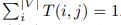 . **Figure 1 **depicts a straightforward example with the states 1 through 4 and the corresponding transition matrix.
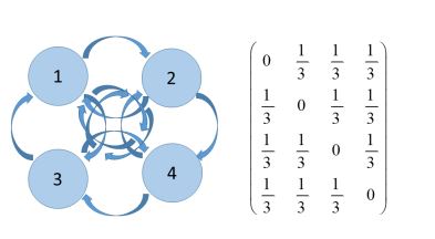
Fig.2 Example Markov Model
This straightforward example can be used to model, for instance, a random walker with four different directions for its steps (left, right, up, and down), each of which has the property of changing its orientation. The following states, with a likelihood of 1/3 given a graphical model and an initial state (for example, 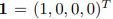 representing the first node), are 2, 3, and 4. Determining a four-dimensional (binary) input and output vector, creating training examples while moving through the network, and using this to train a neural network are obviously nave methods of network training. Unfortunately, a neural network behaves deterministically, meaning that its output is constant for any given input. Alternately, the transition probability of
  can be trained, and a random decision can then be made by sampling from the target distribution. The objective is to convert the predefined statistical behavior of a graphical model to a neural network in order to accommodate non-deterministic behavior and prevent sampling from a target distribution. To do this, we suggest adding an extra value to the input data that contains the random number
  and using a unique learning paradigm, which is described in the following.
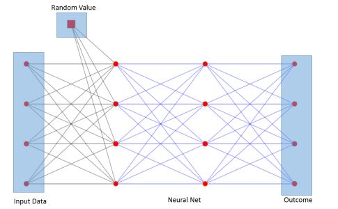
Fig3. Markov Chain Neural Network
Figure 3 shows how the topology is organized. During training and testing, the neural network is connected to the random number as an additional input value. Simply using the above example's five-dimensional input vector (r, 1, 0, 0, 0) or using an additional random bias value along with a random value for the test input can be used to implement it. The crucial concept is that the output vector is guided by the random value in accordance with the predetermined statistical behavior: For a specific training set D with an output vector (or) value) yi,
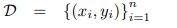
we approximate p(yi|X = xi) as a (in general multivariate) discrete probability distribution. Thus for yi ∈ 1 . . . c, and Y = {y1 . . . yc} and a given input vector X,
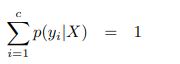
E.g. assuming the transition probabilities from Figure 2, it implies the row-sum to be one. From the training data it is simply approximated as the relative frequency (the empirical probability),
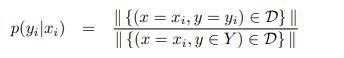
For instance, if the transition probabilities in Figure 2 are assumed, then the row-sum must be 1. It is simply approximated as the relative frequency from the training data (the empirical probability),
Now, an infinite number of input/output pairs can be produced from such a histogram. In order for the distribution of potential output vectors to match the distribution of output vectors in the training data, they reflect a predefined reaction when given a random value as an additional input node. In order to create a distribution of potential outputs, we add an additional random value to the input data vectors.
We accumulate the corresponding cumulative frequency for each potential input state, much like importance sampling, for our simple random walker model and start node  , for example, gaining
  . Then, using a random number generator (r), we create new training data by selecting the best decision from the accumulated interval. The example that follows displays some sample training data produced by this strategy:
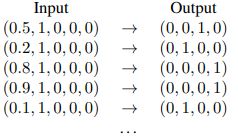
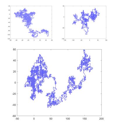
Figure 4 Realizations of different 2D random walks generatedwith a Markov Chain Neural Network
Examples of random walks produced by neural networks are shown in Figure 4 by feeding the output as a new input vector into the network. The images depict the execution of 20.000 steps with the start node (1, 0, 0, 0). Each state has the same likelihood of visitors because the state probability converges to 1/4. Simply put, the additional random value functions as a switch that predetermines the corresponding outcome. For instance, the result for a start node (1, 0, 0, 0) and a random value between [0,1/3] is (0, 1, 0, 0); however, the result for a random value between [1/3,2/3] is (0, 0, 1, 0); etc. Examples of a neural network that produces 3D random walks are shown in Figure 5.
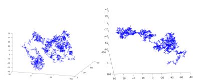
Fig.5 Realizations of different 3D random walks generated with a Markov Chain Neural Network
Conclusion
Markov chains are useful for modeling problems involving random dynamics..The Markov chain can be used to considerably minimize the quantity of data that must be taken into consideration in processes that satisfy the Markov property because knowing the process's past history will not help future predictions. Many applications can be found for it in the fields of science, mathematics, gaming, and information theory.
In conclusion of this article at OpenGenus, this brief introduction only scratches the surface of the immense modeling and computational potential given by Markov chains. These possibilities go well beyond what has been discussed in this introductory material.