In this article at OpenGenus, we will work on predicting bike sharing demand using a dataset provided by University of California, Irvine. The dataset contains count of public bikes rented at each hour in Seoul Bike sharing System with the corresponding Weather data and Holidays information.

Contents:

• Problem Description
• Dataset Description
• Data Preprocessing
• EDA
• Label Encoding
• Checking Multicollinearity
• Regression Plots
• Linear Regression
• Ridge Regression
• Elastic Net Regression
• Decision Tree
• Decision Tree with GridSearchCV
• Random Forest Regressor
• Support Vector Regressor (SVR)
• Gradient Boosting Regressor
• Compare the models
• Conclusion

Problem Description:

With the introduction of rental bikes in urban cities, there has been a substantial improvement in the comfort and convenience of transportation. However, to optimize this system and minimize waiting times, it is vital to make rental bikes available and accessible to the public at the right time. Ensuring a stable supply of rental bikes throughout the city has emerged as a significant concern. To address this challenge, accurate prediction of the number of bikes needed during each hour is crucial.

By accurately forecasting the bike demand, city administrators and bike-sharing operators can plan and allocate resources effectively. This includes ensuring an adequate number of bikes are available during peak hours to meet the surge in demand and avoiding excess inventory during low-demand periods. Moreover, accurate demand prediction enables efficient maintenance and redistribution of bikes, leading to enhanced user satisfaction and optimized operations.

To achieve this, various factors need to be taken into consideration. These factors include weather conditions, such as temperature, humidity, windspeed, visibility, dew point temperature, solar radiation, rainfall, and snowfall. Additionally, other factors like the day of the week, time of the year, holidays, and the functional status of the bike-sharing system are relevant for accurate demand forecasting.

By leveraging historical data and employing advanced predictive modeling techniques, it is possible to develop a robust prediction model that can estimate the bike demand at each hour. Such a model would facilitate proactive decision-making and enable the optimization of resources, ultimately enhancing the overall efficiency and effectiveness of the bike-sharing system in Seoul.

Data Description:

The dataset comprises weather-related information such as temperature, humidity, windspeed, visibility, dew point, solar radiation, snowfall, rainfall, as well as the number of bikes rented per hour and corresponding dates.
Source: https://archive.ics.uci.edu/ml/machine-learning-databases/00560/

Attribute Information:

• Date: The date in the format of year-month-day.
• Rented Bike Count: The count of bikes rented during each hour.
• Hour: The specific hour of the day.
• Temperature: The temperature measured in Celsius.
• Humidity: The relative humidity expressed as a percentage.
• Windspeed: The speed of the wind in meters per second.
• Visibility: The visibility measured in meters.
• Dew Point Temperature: The dew point temperature in Celsius.
• Solar Radiation: The amount of solar radiation in mega joules per square meter.
• Rainfall: The amount of rainfall in millimeters.
• Snowfall: The amount of snowfall in centimeters.
• Seasons: The four seasons of Winter, Spring, Summer, and Autumn.
• Holiday: Indicates whether it is a holiday or a regular day.
• Functional Day: Specifies whether it is a functional (operational) or non-functional hour.

Import necessary libraries

import pandas as pd
import numpy as np
import seaborn as sns
import matplotlib.pyplot as plt
import math
import sklearn
from sklearn.model_selection import train_test_split
from sklearn.preprocessing import MinMaxScaler,StandardScaler
from sklearn.ensemble import RandomForestRegressor,GradientBoostingRegressor
from sklearn.linear_model import Ridge, LinearRegression
from sklearn.svm import SVR
from sklearn.metrics import r2_score,mean_squared_error
from sklearn.tree import DecisionTreeRegressor
from xgboost import XGBRegressor
from sklearn.model_selection import GridSearchCV
from sklearn.ensemble import StackingRegressor
%matplotlib inline

Mount the google drive

from google.colab import drive
drive.mount('/content/drive')

Loading the dataset from google drive

df = pd.read_csv('/content/drive/MyDrive/SeoulBikeData.csv', encoding= 'unicode_escape')

View the head of the dataset

df.head()

Out: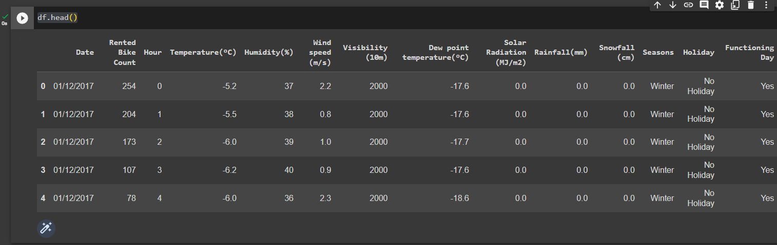

View the tail of the dataset

df.tail()

Out: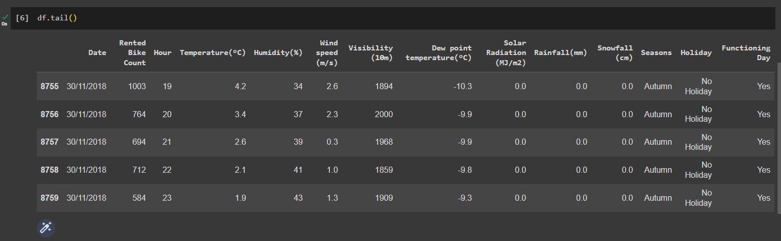

Get the shape of the dataset

print(df.shape())

Out:

View the description of the dataset

df.describe()

Out: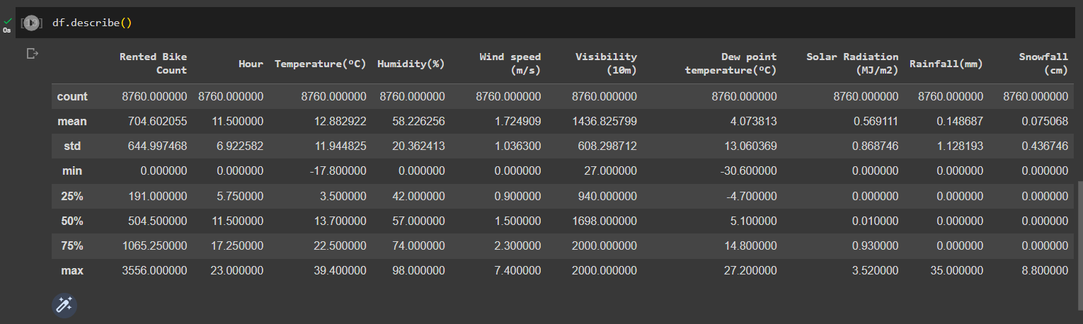

Pre-processing the data

Check the null values in dataset

df.isna().sum()

Out: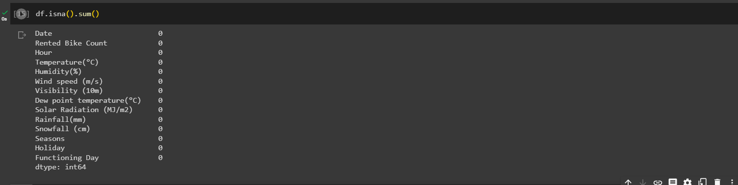

Check duplicate values in dataset

print(len(df[df.duplicated()]))

Out:

Convert the "date" column into three separate columns for "year," "month," and "day,"

import datetime as dt

df['date'] = df['Date'].apply(lambda x: dt.datetime.strptime(x, "%Y-%m-%d"))
df['year'] = df['date'].dt.year
df['month'] = df['date'].dt.month
df['day'] = df['date'].dt.day

# Creating a new column "weekdays_weekend" and dropping the columns "Date," "day," and "year"
df['week'] = df['day'].apply(lambda x: "weekend" if x in ['Saturday', 'Sunday'] else "weekday")
df = df.drop(columns=['Date', 'day', 'year'], axis=1)
df.head()

Out: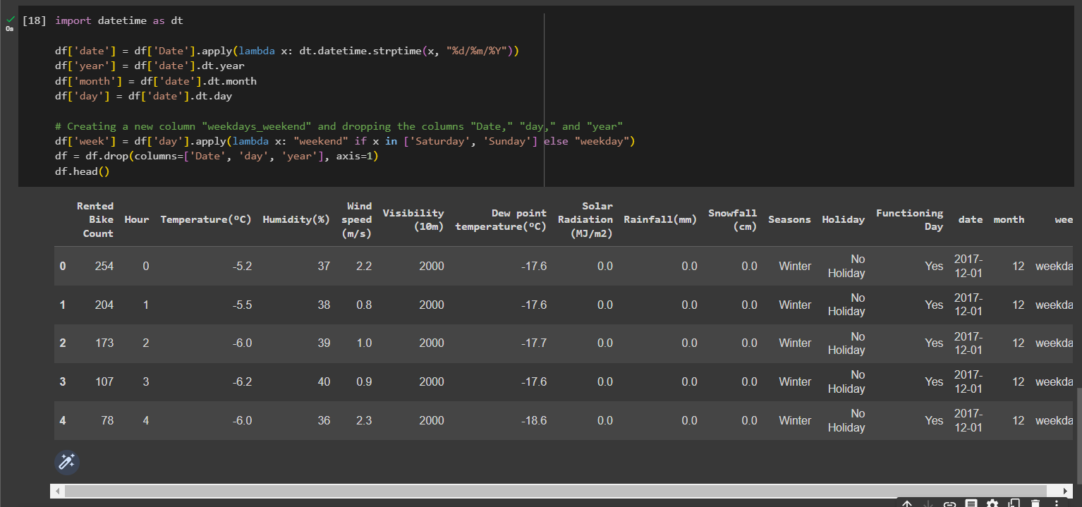

Change int64 columns to category columns

cols=['Hour','month','week']
for col in cols:
  df[col]=df[col].astype('category')

Get a heatmap of co-relation between the features

plt.figure(figsize=(15, 8))
sns.heatmap(df.corr(), annot=True, cmap='coolwarm')
plt.title('Correlation between all the variables', size=16)
plt.show()

Out: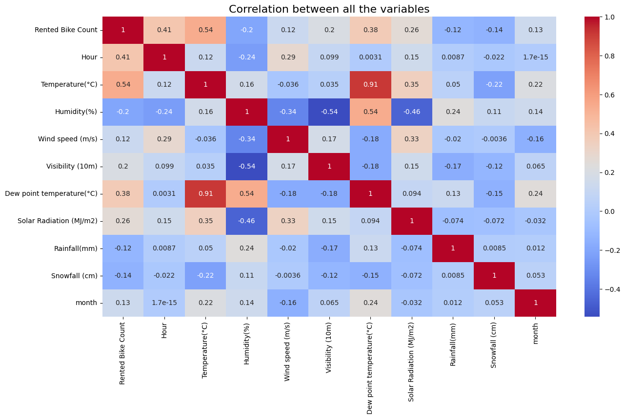

We see that Temperature and Dew point temperature(°C) have high correlation, so dropping them won't affect the outcome of our prediction

df.drop(columns= ['Dew point temperature(°C)'], inplace=True)

Now, we will remove the outliers using the box plot

plt.figure(figsize=(10,10))
for index,item in enumerate([i for i in df.describe().columns.to_list() if i not in ['Rainfall(mm)','Snowfall (cm)']]):
  plt.subplot(3,4,index+1)
  sns.boxplot(df[item])

Out: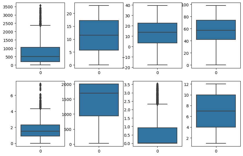

features = list(df.columns)
list_0 = ['Hour', 'Seasons', 'Holiday', 'Functioning Day', 'date', 'month', 'week']
new_features = [x for x in features if x not in list_0]
Q1 = df[new_features].quantile(0.25)
Q3 = df[new_features].quantile(0.75)
IQR = Q3 - Q1
outlier_mask = df[new_features].apply(lambda x: ((x < (Q1.loc[x.name] - 1.5 * IQR.loc[x.name])) | (x > (Q3.loc[x.name] + 1.5 * IQR.loc[x.name]))), axis=0).any(axis=1)
df = df.loc[~outlier_mask]

Handle the null values

df['Temperature(°C)'] = df['Temperature(°C)'].fillna(df['Temperature(°C)'].mean())
df['Humidity(%)'] = df['Humidity(%)'].fillna(df['Humidity(%)'].mean())
df['Wind speed (m/s)'] = df['Wind speed (m/s)'].fillna(df['Wind speed (m/s)'].mean())
df['Visibility (10m)'] = df['Visibility (10m)'].fillna(df['Visibility (10m)'].mean())

df['Solar Radiation (MJ/m2)'] = df['Solar Radiation (MJ/m2)'].fillna(df['Solar Radiation (MJ/m2)'].mean())
df['Rainfall(mm)'] = df['Rainfall(mm)'].fillna(df['Rainfall(mm)'].mean())
df['Snowfall (cm)'] = df['Snowfall (cm)'].fillna(df['Snowfall (cm)'].mean())

EDA

Monthly analysis

fig,ax=plt.subplots(figsize=(10,5))
sns.barplot(data=df,x='month',y='Rented Bike Count',ax=ax,capsize=.2)
ax.set(title='Count of Rented bikes according to month ')

Out: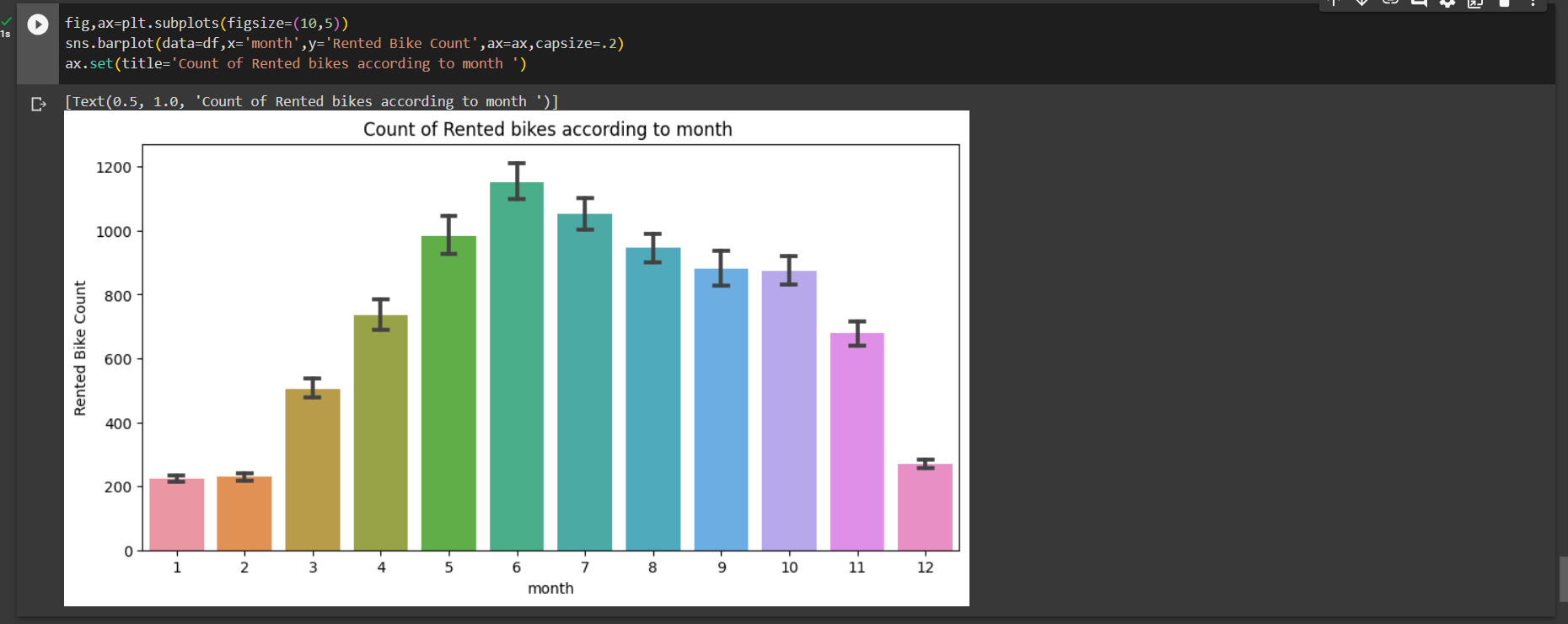
We can say that the demand of bikes from month 5 to month 10 is quite high.

Time analysis

fig,ax=plt.subplots(figsize=(20,8))
sns.pointplot(data=df,x='Hour',y='Rented Bike Count',hue='week',ax=ax)
ax.set(title='Count of Rented bikes acording to weekdays_weekend ')

Out: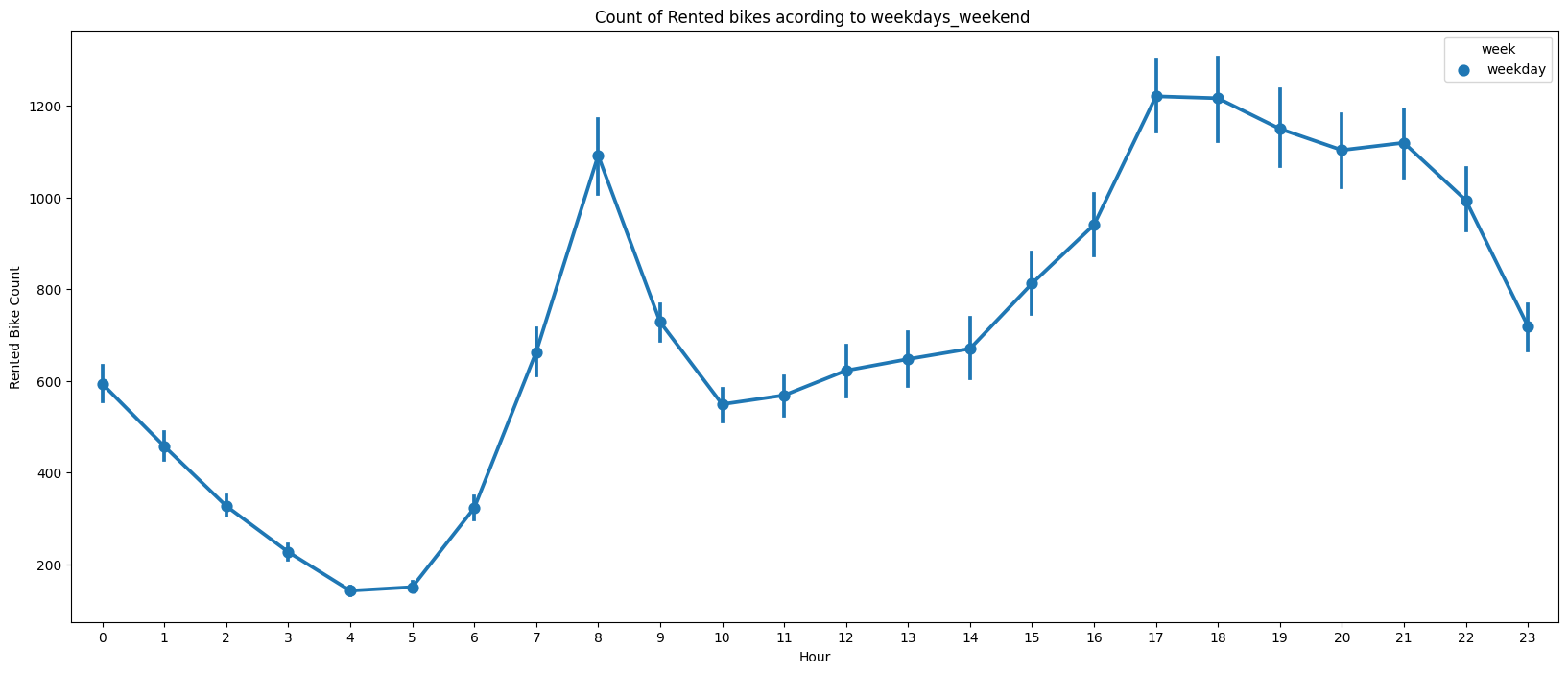
We can see that the peak time are 7 am to 9 am and 5 pm to 7 pm.

Season analysis

fig,ax=plt.subplots(figsize=(15,8))
sns.boxplot(data=df,x='Seasons',y='Rented Bike Count',ax=ax)
ax.set(title='Count of Rented bikes acording to Seasons ')

Out: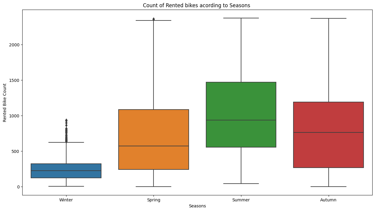

fig,ax=plt.subplots(figsize=(15,8))
sns.barplot(data=df,x='Seasons',y='Rented Bike Count',ax=ax,capsize=.2)
ax.set(title='Count of Rented bikes acording to Seasons ')

Out: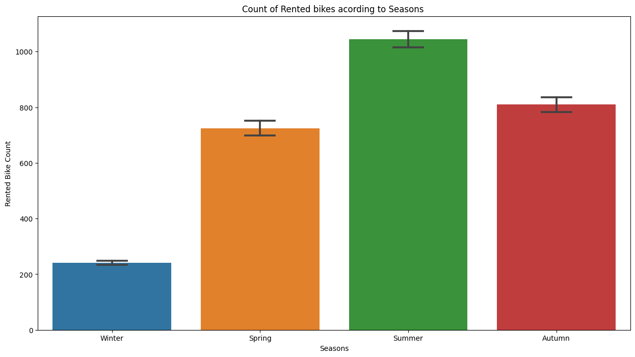
We see that in summer season the use of rented bike is high In winter season the use of rented bike is very low because of snowfall.

Count of rented bikes in different visibilities

df_visi = pd.DataFrame(df.groupby('Visibility (10m)')['Rented Bike Count'].sum())
df_visi.reset_index(inplace=True)
plt.figure(figsize=(8,6))
sns.distplot(df_visi['Visibility (10m)'])

Out: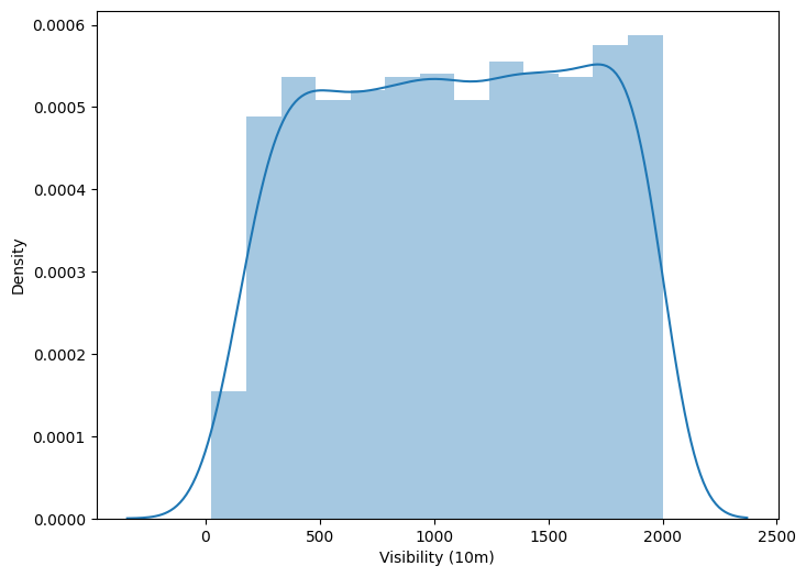
People tend to rent bikes when the visibility is between 300 to 1700.

Label encoding

creating dummy variables for categorical feature which are Seasons, month, DayOfWeek, year, fuctioning day, holiday.

seasons = pd.get_dummies(df['Seasons'])
working_day = pd.get_dummies(df['Holiday'])
F_day = pd.get_dummies(df['Functioning Day'])
month = pd.get_dummies(df['month'])
week_day = pd.get_dummies(df['week'])
df = pd.concat([df,seasons,working_day,F_day,month,week_day],axis=1)
df.head()

Out: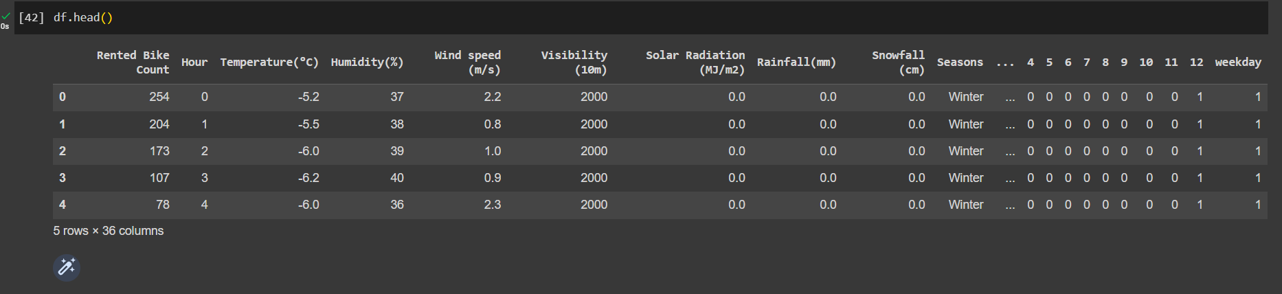

dropping columns for which dummy variables were created

df.drop(['Seasons','Holiday','Functioning Day','week','month'],axis=1,inplace=True)

Checking multicollinearity

Checking multicollinearity is an important step in regression analysis to assess the presence and severity of collinearity among predictor variables. Collinearity refers to a high correlation between two or more independent variables in a regression model.
High multicollinearity can cause several issues in regression analysis, including:

• Unstable and unreliable coefficient estimates
• Difficulty in interpreting the model
• Reduced model efficiency

To check for multicollinearity, various techniques can be used, and one common approach is calculating the Variance Inflation Factor (VIF). The VIF quantifies the extent to which a predictor variable can be explained by other predictor variables. It measures the correlation between a predictor variable and the other predictors in the model.

calculating multicollinearity

from statsmodels.stats.outliers_influence import variance_inflation_factor
# Select only numeric columns for VIF calculation
numeric_columns = df.select_dtypes(include='number')
# Calculate VIF for each feature
vif_data = pd.DataFrame()
vif_data["feature"] = numeric_columns.columns
vif_data["VIF"] = [variance_inflation_factor(numeric_columns.values, i)
                   for i in range(len(numeric_columns.columns))]
vif_data['VIF'] = round(vif_data['VIF'], 2)
print(vif_data)

Out: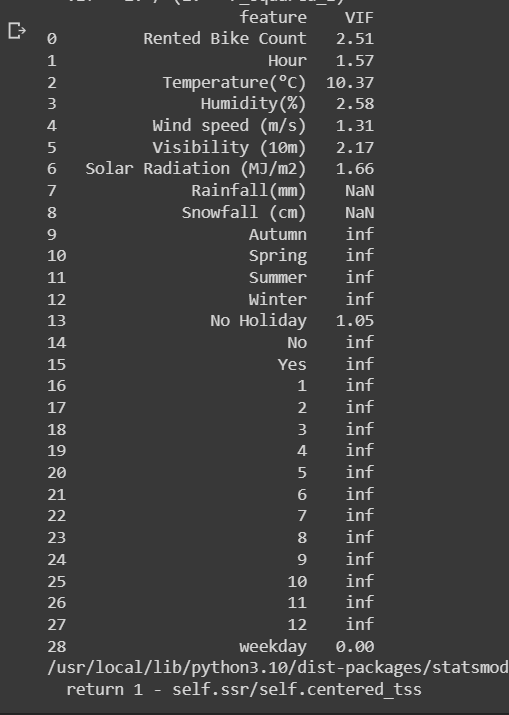

By examining the VIF values, one can identify highly correlated variables and take appropriate actions to address multicollinearity. These actions may include:

• Removing one or more correlated variables from the model.
• Combining correlated variables into a single composite variable.
• Gathering more data to improve the independence of the predictors.

df=df.drop(['Rainfall(mm)','Snowfall (cm)'],axis=1)

Regression Plots

Getting regression plots for all the numerical features

# Select numerical columns
numerical_columns = df.select_dtypes(include='number')

# Calculate the number of subplots to create
num_plots = min(len(numerical_columns), 6)

# Determine the number of rows and columns for the subplot grid
num_rows = (num_plots - 1) // 2 + 1
num_cols = min(num_plots, 2)

# Set up the grid of subplots
fig, axes = plt.subplots(nrows=num_rows, ncols=num_cols, figsize=(12, 4 * num_rows))

# Flatten the axes array
axes = axes.flatten()

# Plot regression plots for each numerical column
for i in range(num_plots):
    col = numerical_columns.columns[i]
    sns.regplot(x=df[col], y=df['Rented Bike Count'], scatter_kws={"color": 'orange'}, line_kws={"color": "black"}, ax=axes[i])
    axes[i].set_xlabel(col)
    axes[i].set_ylabel('Rented Bike Count')

# Remove any unused subplots
for j in range(num_plots, num_rows * num_cols):
    fig.delaxes(axes[j])

# Adjust spacing between subplots
plt.tight_layout()

# Display the plot
plt.show()

Out: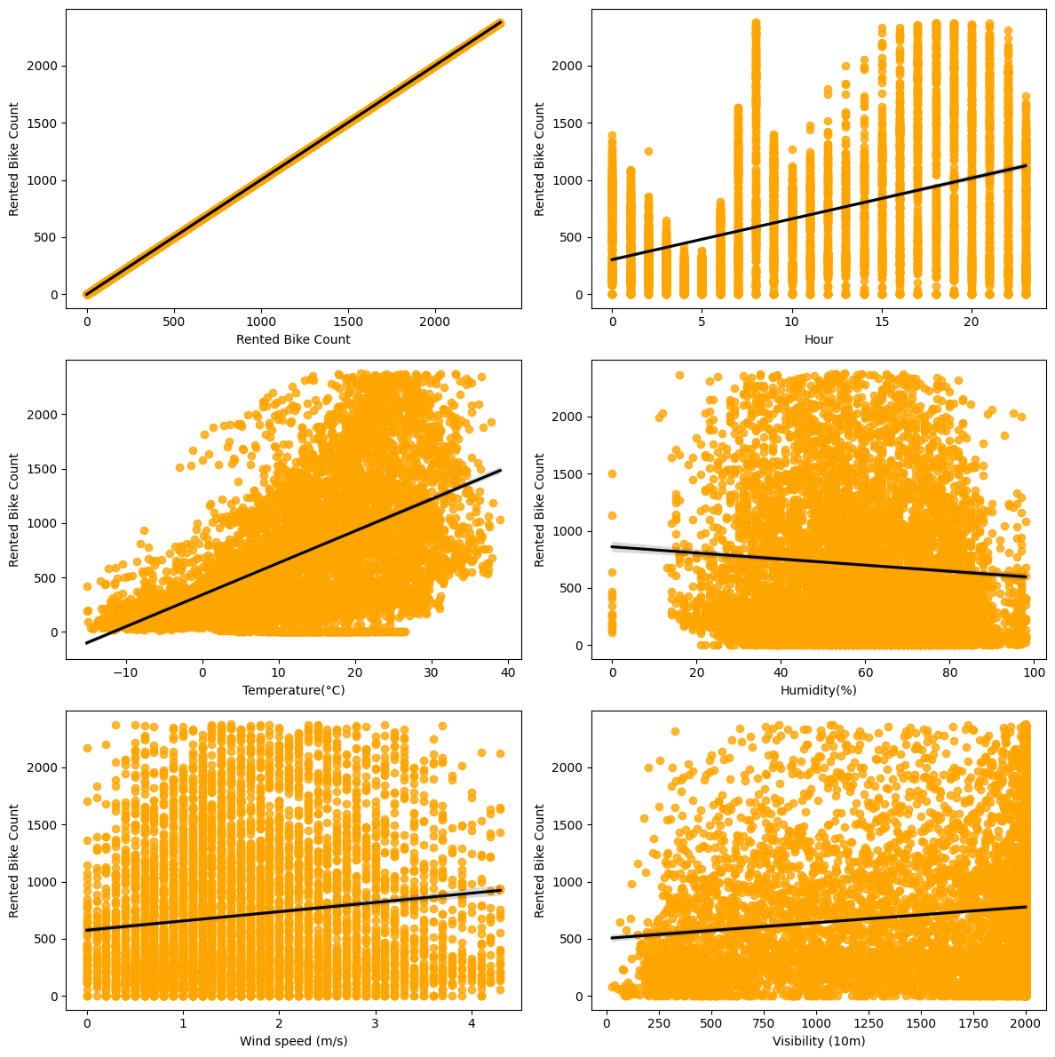

Create train and test data

X = df.drop(columns=['Rented Bike Count'], axis=1)
y = np.sqrt(df['Rented Bike Count'])
X['date'] = (X['date'] - np.datetime64('1970-01-01T00:00:00Z')) / np.timedelta64(1, 's')
from sklearn.model_selection import train_test_split
from sklearn.preprocessing import StandardScaler

# Convert feature/column names to strings
X.columns = X.columns.astype(str)

# Split the data into train and test sets
X_train, X_test, y_train, y_test = train_test_split(X, y, test_size=0.25, random_state=0)
print(X_train.shape)
print(X_test.shape)

# Convert feature/column names to strings
X_train.columns = X_train.columns.astype(str)
X_test.columns = X_test.columns.astype(str)

# Standardize the independent variables
scaler = StandardScaler()
X_train = scaler.fit_transform(X_train)
X_test = scaler.transform(X_test)

Perform Linear Regression

Linear regression is a widely used statistical modeling technique that aims to establish a linear relationship between a dependent variable (target variable) and one or more independent variables (predictor variables). It assumes that this relationship can be approximated by a straight line.

The fundamental idea behind linear regression is to find the best-fitting line that represents the relationship between the predictor variables and the target variable. This line is determined by estimating the coefficients (slope and intercept) that minimize the differences between the observed values and the predicted values.

Import packages and get score

from sklearn.linear_model import LinearRegression
reg= LinearRegression().fit(X_train, y_train)
reg.score(X_train, y_train)

Out: 0.6922990275319361

Regression coefficient

reg.coef_

Out:
array([ 3.76850533e+00, 5.49494568e+00, -1.62642730e+00, 3.46111463e-01,
3.15722144e-01, -1.91279044e-03, -1.44268068e+00, 1.29494497e+00,
-4.37606601e-02, 1.80337571e-01, -1.46987357e+00, 7.01458266e-01,
-2.75168791e+00, 2.75168791e+00, -8.71158391e-01, -9.30950769e-01,
-7.51345212e-01, -8.11229410e-02, 8.15360021e-01, 9.26195820e-01,
-3.15840674e-02, -5.53401502e-01, 1.65427712e-01, 1.03465920e+00,
7.77617563e-01, -4.90103053e-01, 0.00000000e+00])

Calculate the errors

y_pred_train=reg.predict(X_train)
y_pred_test=reg.predict(X_test)
from sklearn.metrics import mean_squared_error, mean_absolute_error, r2_score

# Calculate MSE
MSE_lr = mean_squared_error(y_train, y_pred_train)
print("MSE:", MSE_lr)

# Calculate RMSE
RMSE_lr = np.sqrt(MSE_lr)
print("RMSE:", RMSE_lr)

# Calculate MAE
MAE_lr = mean_absolute_error(y_train, y_pred_train)
print("MAE:", MAE_lr)

# Calculate R2
r2_lr = r2_score(y_train, y_pred_train)
print("R2:", r2_lr)

# Calculate adjusted R2
Adjusted_R2_lr = (1 - (1 - r2_score(y_train, y_pred_train)) * ((X_test.shape[0] - 1) / (X_test.shape[0] - X_test.shape[1] - 1)))

print("Adjusted R2:", Adjusted_R2_lr)

Out: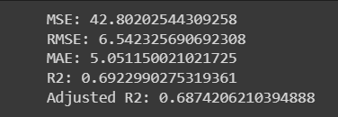

Ridge Regression

Now, we'll perform linear regression with L2 regularization which is also called Ridge regression.

Ridge regression is a regularization technique used in linear regression to address the issue of multicollinearity and to prevent overfitting. It is an extension of ordinary least squares (OLS) regression that introduces a penalty term to the cost function, allowing for a balance between fitting the training data and reducing the complexity of the model.

The idea behind ridge regression is to add a penalty term to the sum of squared residuals in the cost function. This penalty term is proportional to the square of the magnitude of the coefficients (weights) of the regression model. By adding this term, ridge regression shrinks the coefficients towards zero, effectively reducing their magnitude.

from sklearn.linear_model import Ridge
from sklearn.metrics import mean_squared_error, r2_score

# Create and train the Ridge model
ridge = Ridge(alpha=0.1)
ridge.fit(X_train, y_train)

# Make predictions on training and test data
y_pred_train_ridge = ridge.predict(X_train)
y_pred_test_ridge = ridge.predict(X_test)

# Evaluate metrics
# Calculate MSE
MSE = mean_squared_error(y_test, y_pred_test_ridge)
print("MSE:", MSE)

# Calculate RMSE
RMSE = np.sqrt(MSE)
print("RMSE:", RMSE)

# Calculate R2
r2_ridge_test = r2_score(y_test, y_pred_test_ridge)
print("R2:", r2_ridge_test)

# Calculate adjusted R2
adjusted_r2 = 1 - (1 - r2_score(y_test, y_pred_test_ridge)) * ((X_test.shape[0] - 1) / (X_test.shape[0] - X_test.shape[1] - 1))
print("Adjusted R2:", adjusted_r2)

Out: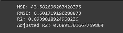

In this code, the Ridge model is created and trained using X_train and y_train. Then, predictions are made on both the training and test data. Metrics such as MSE, RMSE, R2, and adjusted R2 are calculated based on the predicted values y_pred_test_ridge and the actual target values y_test. The results are printed accordingly.

Ridge regression is a useful technique when dealing with datasets that exhibit multicollinearity, where predictor variables are highly correlated. By introducing a regularization term, ridge regression helps to stabilize the model and avoid overfitting. It provides a balance between fitting the training data and reducing model complexity, making it a valuable tool in predictive modeling tasks.

With elastic net

Elastic Net is a regularization technique used in linear regression to handle multicollinearity and prevent overfitting. It combines both L1 (Lasso) and L2 (Ridge) regularization penalties, offering a balance between feature selection and coefficient shrinkage.

The idea behind Elastic Net is to add two penalty terms to the cost function: the L1 penalty, which encourages sparsity by promoting some coefficients to become exactly zero, and the L2 penalty, which shrinks the coefficients towards zero. The relative contribution of each penalty is controlled by a parameter called alpha.

In this code, the ElasticNet model is created and trained using X_train and y_train. Then, predictions are made on both the training and test data. Metrics such as MSE, RMSE, MAE, R2, and adjusted R2 are calculated based on the predicted values y_pred_train_en and the actual target values y_train. The results are printed accordingly.

from sklearn.linear_model import ElasticNet
from sklearn.metrics import mean_squared_error, mean_absolute_error, r2_score

# Create and train the ElasticNet model
elasticnet = ElasticNet(alpha=0.1, l1_ratio=0.5)
elasticnet.fit(X_train, y_train)

# Make predictions on training and test data
y_pred_train_en = elasticnet.predict(X_train)
y_pred_test_en = elasticnet.predict(X_test)

# Evaluate metrics
# Calculate MSE
MSE_e = mean_squared_error(y_train, y_pred_train_en)
print("MSE:", MSE_e)

# Calculate RMSE
RMSE_e = np.sqrt(MSE_e)
print("RMSE:", RMSE_e)

# Calculate MAE
MAE_e = mean_absolute_error(y_train, y_pred_train_en)
print("MAE:", MAE_e)

# Calculate R2
r2_e = r2_score(y_train, y_pred_train_en)
print("R2:", r2_e)

# Calculate adjusted R2
adjusted_r2_e = 1 - (1 - r2_score(y_train, y_pred_train_en)) * ((X_test.shape[0] - 1) / (X_test.shape[0] - X_test.shape[1] - 1))
print("Adjusted R2:", adjusted_r2_e)

Out: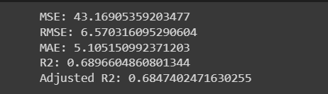

Elastic Net is particularly useful when dealing with datasets that have a large number of features and exhibit multicollinearity. It allows for automatic feature selection by driving some coefficients to zero while also providing shrinkage to reduce the impact of irrelevant features. By finding the right balance between L1 and L2 regularization, Elastic Net offers a flexible and effective approach for regression tasks.

Decision Tree

Decision Tree is a non-parametric supervised learning algorithm used for both regression and classification tasks. It makes predictions by recursively partitioning the data based on feature values, creating a hierarchical structure resembling a tree.

from sklearn.tree import DecisionTreeRegressor
from sklearn.metrics import r2_score

# Create and train the Decision Tree regressor
regressor = DecisionTreeRegressor(random_state=0)
regressor.fit(X_train, y_train)

# Make predictions on training and test data
y_pred_train = regressor.predict(X_train)
y_pred_test = regressor.predict(X_test)

# Calculate R2 score for training and test data
r2_train = r2_score(y_pred_train, y_train)
r2_test = r2_score(y_pred_test, y_test)

# Print the R2 score for test data (DT)
print("DT R2 Score:", r2_test)

Out: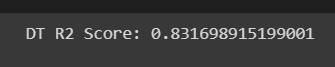

Decision Trees are intuitive and can handle both numerical and categorical features. They are capable of capturing non-linear relationships and interactions between variables. However, they can be prone to overfitting, especially when the tree grows too deep or the dataset contains noisy or irrelevant features. Techniques like pruning, ensemble methods (e.g., Random Forest, Gradient Boosting), and regularization can be used to address these limitations.

Decision tree with GridSearchCV

from sklearn.tree import DecisionTreeRegressor
from sklearn.model_selection import GridSearchCV
from sklearn.metrics import r2_score

# Create the Decision Tree regressor
regressor = DecisionTreeRegressor(random_state=0)

# Define the hyperparameter grid
param_grid = {'max_depth': [1, 4, 5, 6, 7, 10, 15, 20, 8]}

# Perform GridSearchCV to find the best hyperparameters
regressor_gs_cv = GridSearchCV(regressor, param_grid, scoring='r2', cv=5)
regressor_gs_cv.fit(X_train, y_train)

# Get the best estimator found by GridSearchCV
best_estimator = regressor_gs_cv.best_estimator_

# Calculate the R2 score for the test data with the best parameters
r2_score_dt = r2_score(y_pred_test, y_test)

# Calculate the R2 score for the test data with hyperparameter tuning
r2_score_dt_tuned = regressor_gs_cv.score(X_test, y_test)

# Print the R2 scores
print(f"The R2 score of the Decision Tree is: {r2_score_dt}")
print(f"The R2 score of the Decision Tree with hyperparameter tuning is: {r2_score_dt_tuned}")

Out:

Random Forest Regressor

Random Forest Regressor is an ensemble learning algorithm based on the concept of decision trees. It combines multiple decision trees to create a more robust and accurate predictive model.

from sklearn.ensemble import RandomForestRegressor
from sklearn.metrics import mean_squared_error, r2_score
import matplotlib.pyplot as plt
import seaborn as sns

# Create the Random Forest regressor
rf_reg = RandomForestRegressor(n_estimators=1000, random_state=5)

# Train the model
rf_reg.fit(X_train, y_train)

# Make predictions
pred_train = rf_reg.predict(X_train)
pred_test = rf_reg.predict(X_test)

# Calculate MSE for the training set
MSE_train = mean_squared_error(y_train, pred_train)
print(f"MSE (Train): {MSE_train}")

# Calculate RMSE for the training set
RMSE_train = np.sqrt(MSE_train)
print(f"RMSE (Train): {RMSE_train}")

# Calculate R2 score for the training set
R2_score_train = r2_score(y_train, pred_train)
print(f"R2 Score (Train): {R2_score_train}")

# Calculate MSE for the test set
MSE_test = mean_squared_error(y_test, pred_test)
print(f"MSE (Test): {MSE_test}")

# Calculate RMSE for the test set
RMSE_test = np.sqrt(MSE_test)
print(f"RMSE (Test): {RMSE_test}")

# Calculate R2 score for the test set
R2_score_test = r2_score(y_test, pred_test)
print(f"R2 Score (Test): {R2_score_test}")

Out: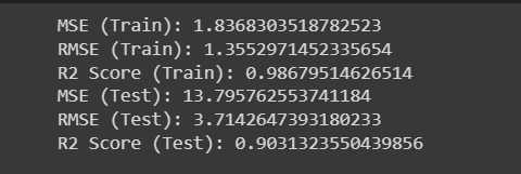

Random Forest Regressor is known for its ability to handle complex datasets, capture non-linear relationships, and handle high-dimensional feature spaces. It is less prone to overfitting compared to individual decision trees and can provide more robust and accurate predictions.

SVR

Support Vector Regressor (SVR) is a machine learning algorithm that is used for regression tasks. It is based on the idea of Support Vector Machines (SVM) and extends it to handle regression problems.

from sklearn.svm import SVR
from sklearn.model_selection import GridSearchCV
from sklearn.metrics import mean_absolute_error, mean_squared_error, r2_score

# Selecting the values of SVR
param = {
    'C': [1, 5, 10],
    'degree': [3, 8],
    'coef0': [0.01, 10, 0.5],
    'gamma': ('auto', 'scale')
}

# Train the model
model_svr = SVR(kernel='rbf')
grid_search = GridSearchCV(model_svr, param, cv=3)
grid_search.fit(X_train, y_train)

# Predicting for both train and test sets
y_pred_train = grid_search.predict(X_train)
y_pred_test = grid_search.predict(X_test)

# Finding each of the metrics for the training set
print('Training Set Metrics:')
print('MAE:', mean_absolute_error(y_train, y_pred_train))
print('MSE:', mean_squared_error(y_train, y_pred_train))
print('R2 Score:', r2_score(y_train, y_pred_train))

# Finding each of the metrics for the test set
print('\nTest Set Metrics:')
print('MAE:', mean_absolute_error(y_test, y_pred_test))
print('MSE:', mean_squared_error(y_test, y_pred_test))
print('R2 Score:', r2_score(y_test, y_pred_test))

Out: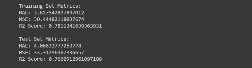

SVR is particularly useful when dealing with non-linear regression problems and datasets with complex relationships. It has the ability to handle high-dimensional feature spaces and is less affected by outliers compared to some other regression algorithms. By finding an optimal hyperplane, SVR aims to generalize well on unseen data and make accurate predictions.

Gradient Boosting Regressor

Gradient Boosting Regressor is a machine learning algorithm that combines multiple weak prediction models, typically decision trees, to create a strong predictive model.

from sklearn.model_selection import GridSearchCV
from sklearn.ensemble import GradientBoostingRegressor
from sklearn.metrics import r2_score

# Define the hyperparameters
param_dict = {
    'n_estimators': [50, 80, 100],
    'max_depth': [4, 6, 8],
    'min_samples_split': [50, 100, 150],
    'min_samples_leaf': [40, 50]
}

# Create an instance of the GradientBoostingRegressor
gb_model = GradientBoostingRegressor()

# Perform grid search
gb_grid = GridSearchCV(estimator=gb_model, param_grid=param_dict, cv=5, verbose=2)
gb_grid.fit(X_train, y_train)

# Get the best estimator and best parameters
best_estimator = gb_grid.best_estimator_
best_params = gb_grid.best_params_

# Make predictions on train and test data
y_pred_train = best_estimator.predict(X_train)
y_pred_test = best_estimator.predict(X_test)

# Evaluate the model
r2_train = r2_score(y_train, y_pred_train)
r2_test = r2_score(y_test, y_pred_test)

print('Best Parameters:', best_params)
print('R2 Score (Train):', r2_train)
print('R2 Score (Test):', r2_test)

Out:

Visualizing the results

sns.scatterplot(x=y_pred_test,y=y_test)
plt.title('Predicted vs Actual - gradientBoosting')
plt.ylabel('Predicted values')
plt.xlabel('Actual Values')

Out: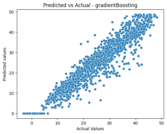

Gradient Boosting Regressor is known for its ability to handle complex relationships and nonlinear patterns in the data. By combining multiple weak learners, it creates a strong model that can make accurate predictions. It is widely used in various regression problems and has gained popularity due to its effectiveness and robustness.

Compare the models with R2 scores

models = ['Ridge_model', 'elasticnet', 'Decision_Tree_model', 'Decision_Tree_model_gridcv', 'random_forest', 'SVR', 'gradient']
R2_value = [r2_ridge_test, r2_e, r2_test, r2_score_dt_tuned, R2_score_test, svr, r2_test_1]

compare_models = pd.DataFrame([R2_value], columns=models, index=['r2_value'])
compare_models

Out:

Execution

For using this model, run the Seoul_bike_prediction.ipynb provided at

https://github.com/deshpanda/Bike-Sharing-Demand-Prediction-Seoul.

Conclusion

After analyzing the dataset, we have made several observations:

Hour of the day holds the most importance among all the features for predicting the number of bike rentals.

• The highest number of bike rentals occurs during the Autumn/Fall and Summer seasons, while the lowest occurs during the Spring season.

• Clear weather conditions are associated with the highest number of bike rentals, while snowy or rainy conditions are associated with the lowest.

• The top 5 important features for predicting bike rentals are Season_winter, Temperature, Hour, Season_autumn, and Humidity.

• There is a significant decrease in bike rentals on non-functioning days.

• People tend to rent bikes when the temperature ranges from -5 to 25 degrees Celsius.

• Visibility between 300 to 1700 meters also influences bike rental demand.

• Based on our experiments, we can conclude that gradient boosting and random forest regressors, with the use of hyperparameters, provide the best results for predicting the number of bike rentals.