
Get this book -> Problems on Array: For Interviews and Competitive Programming
In this article, we will be learning about an important step in the machine learning process: feature engineering.
Table of Contents
- Introduction
- Installation/Setup
- Loading the Dataset
- Feature Generation and Transformation
- Mathematical Transforms
- Parsing Complex Data Types
- Binning
- Scaling
- Determining Feature Importance Using Mutual Information
- Testing and Results
- Conclusion
Introduction
The goal of feature engineering is to make data better for the problem you are trying to solve using machine learning.
Feature engineering can help enhance a model's performance by producing new features and determining which features are important for the prediction task. Through data transformations, the model can learn relationships that weren't present in the original data.
There are no set rules for what feature engineering techniques work best in general. Datasets vary a lot, so sometimes certain techniques will be more useful than others, but other times they may not. Feature engineering is a trial-and-error process - it involves a lot of experimentation regarding what features to create and transform and deciding which features to remove.
We will first discuss different feature engineering techniques and then walk through an example using the July 2021 Tabular Series Playground Kaggle Competition.
Feature Generation and Transformation
We can apply a series of transformations on existing features to generate new features. This process adds new information and it may result in a more accurate model. We will be going over the following feature generation and transformation techniques:
- Mathematical transforms (applying arithmetic operations)
- Parsing and breaking down complex data types (eg. dates, times, etc.),
- Binning
- Scaling
We will be going over each of these in more depth and we will also learn how to implement them in Python. The Pandas library makes it very simple to perform most of these transformations.
Mutual Information
Mutual Information is a way to determine how important a feature is by measuring the relationship between each feature and the target variable. It describes relationships in terms of uncertainty, where the mutual information between two quantities measures how much uncertainty about a variable is reduced by having knowledge about the other variable.
Mutual information is a great general-purpose metric. It is easy to use, efficient, and it is able to detect any kind of relationship, not just linear.
The least possible mutual information between any two quantities is 0. When it is zero, that means there is no relationship between the two quantities. For our purposes, a feature that has a mutual information score of zero or very close to 0 is likely an unimportant feature that does not help model performance. Unimportant features may even negatively impact model performance.
There is no maximum mutual information, but values are usually less than 2. Higher mutual information corresponds with more important features.
Installation/Setup
For this article, we will need Pandas, NumPy, and Scikit-Learn. We can install them using the pip package manager:
pip install pandas
pip install numpy
pip install scikit-learn
In case the commands above do not work, please see the following links for specific installation instructions:
Import the necessary libraries:
import numpy as np
import pandas as pd
from sklearn.ensemble import RandomForestRegressor
from sklearn.feature_selection import mutual_info_regression
from sklearn.metrics import mean_squared_error
from sklearn.model_selection import train_test_split
from sklearn.preprocessing import StandardScaler
Loading the Dataset
We will be using the dataset from the July 2021 Tabular Series Playground Kaggle Competition, as it contains different kinds of features for us to apply feature engineering techniques on. We will use the file named "train.csv".
df = pd.read_csv("train.csv")
Let's take a look at the first few rows of the dataset:
df.head()
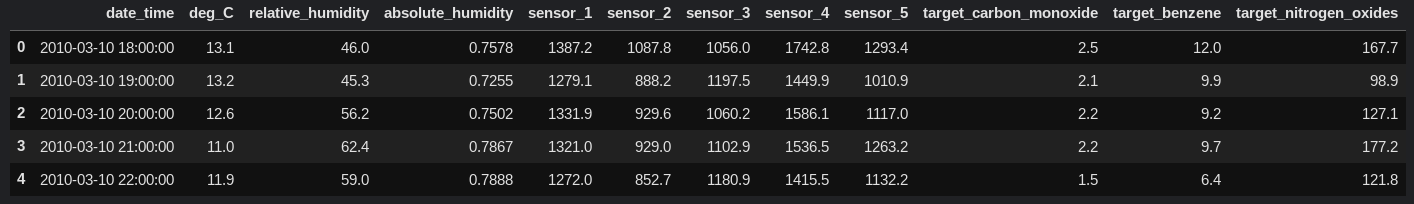
There are three target values for our model to predict: target_carbon_monoxide, target_benzene, and target_nitrogen_oxides.
Feature Generation and Transformation
We will create several new features, and we will later remove the ones that are unimportant.
Mathematical Transforms
We can apply a series of arithmetic operations to our data. These operations are very simple to perform using Pandas. Pandas allows us to treat columns as ordinary variables.
Here are some examples:
df['temp_plus_humidity'] = df['deg_C'] + df['relative_humidity']
df['temp_minus_humidity'] = df['deg_C'] - df['relative_humidity']
df['temp_times_humidity'] = df['deg_C'] * df['relative_humidity']
df['temp_divided_by_humidity'] = df['deg_C'] / df['relative_humidity']
df.head()
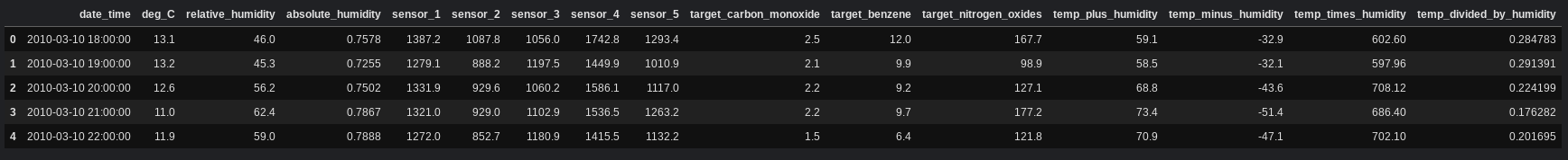
As we can see above, the columns have been created. Each of the new columns stores the result of the operation for each sample in the columns deg_C and relative_humidity. For example, the first row in the dataset has contains 13.1 for deg_C and 46.0 for relative_humidity. The column temp_plus_humidity for that row contains 59.1, which is equivalent to 13.1 + 46.0.
The goal of feature engineering is to create meaningful features. The code above demonstrated how we could apply mathematical transforms, but we can create more meaningful features by doing some research on the data we're given and understanding how we can use the given information to determine something else.
For example, we can use the columns relative_humidity and absolute_humidity to determine the maximum amount of water vapor the air could contain at the current temperature. Absolute humidity measures the total amount of water vapor present in a given volume of air, and relative humidity is defined as the amount of water vapor present in the air divided by the maximum amount of water vapor the air could contain at the current temperature. Since we're given both the absolute humidity and relative humidity, we can calculate the maximum amount of water vapor the air could contain by dividing the absolute humidity by the relative humidity.
df['max_water_vapor'] = df['absolute_humidity'] / (df['relative_humidity'] / 100) # we are dividing by the percentage
Using mathematical transforms, we can also convert Celsius into Fahrenheit. The formula to convert from Celsius to Fahrenheit is given by the following equation:
°F = (9/5)°C+32
Here's how that translates into code:
df['deg_F'] = df['deg_C'] * 9/5 + 32
Parsing Complex Data Types
Not all datasets consist only of numbers. They can contain more complex data types such as strings and dates/times. Most machine learning models won't accept these data types as input, however, so we must process these data types to pass them in a format that can be understood by machine learning models.
Parsing Date and Time
The column date_time contains a timestamp of when each row's data was measured. We cannot directly use this column as input to a model, but we can parse it so that a model will be able to use it.
Let's take a look at the column's data type, or dtype:
print(df['date_time'].dtype)
object
"Object" means that the column is currently in string format.
Pandas provides a helpful method called to_datetime, which can convert a string into a datetime object. The following code creates a new column called date_time_parsed:
df['date_time_parsed'] = pd.to_datetime(df['date_time'], infer_datetime_format=True)
The parameter infer_datetime_format is True so that Pandas can automatically determine the date and time format. This way, we don't need to specify the format.
When we check the dtype of the date_time_parsed column, we can see that the new column has successfully parsed the strings into datetime objects:
print(df["date_time_parsed"].dtype)
datetime64[ns]
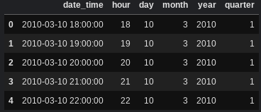
We won't be passing this column into the model, but we can use this column to generate numerical features:
df['hour'] = df['date_time_parsed'].dt.hour # gets the hour of day
df['day'] = df['date_time_parsed'].dt.day # gets the day
df['month'] = df['date_time_parsed'].dt.month # gets the month of the year
df['year'] = df['date_time_parsed'].dt.year # gets the year
df['quarter'] = df['date_time_parsed'].dt.quarter # gets the quarter of the year (ranges from 1-4)
Now, let's take a look at the updated columns:
df[["date_time", 'hour', "day", "month", "year", "quarter"]].head()
Binning
Binning is a way to group continuous values into a smaller number of "bins", each of which represents a certain range of values. This creates new categorical features that represent which range or "bin" a value belongs to.
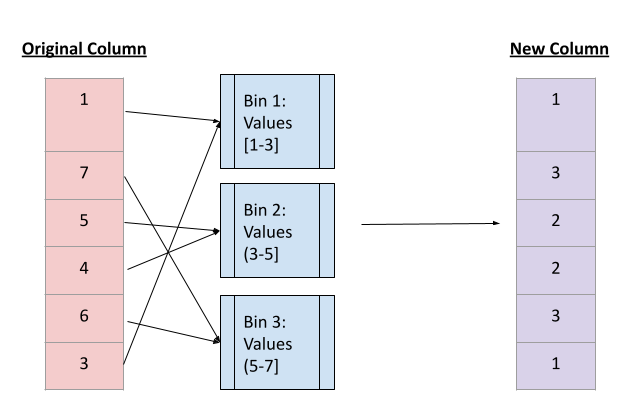
This image gives a visual representation of what binning does. Image created by author.
Pandas provides a cut method that is used to bin data. In the following code example, we will separate all the sensor data into 5 bins of equal size and output the range of values for each bin.
for i in range(5):
    # retbins = True returns the bins so we can access the range of values
    df[f'binned_sensor_{i+1}'], bins = pd.cut(df[f'sensor_{i+1}'], 5, retbins=True, labels=False)
    print(f'Bins for sensor {i+1} :{bins}')
Bins for sensor 1 :[ 618.832  913.9   1207.5   1501.1   1794.7   2088.3  ]
Bins for sensor 2 :[ 362.0614  751.72   1139.44   1527.16   1914.88   2302.6   ]
Bins for sensor 3 :[ 308.3432  761.96   1213.32   1664.68   2116.04   2567.4   ]
Bins for sensor 4 :[ 550.5391 1025.08   1497.26   1969.44   2441.62   2913.8   ]
Bins for sensor 5 :[ 240.3481  713.08   1183.46   1653.84   2124.22   2594.6   ]
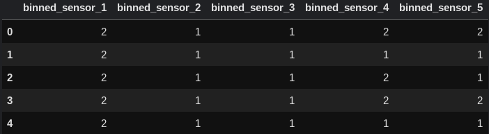
Let's take a look at the new columns we created:
df[["binned_sensor_1", "binned_sensor_2", "binned_sensor_3", "binned_sensor_4", "binned_sensor_5"]].head()
Scaling
Feature scaling helps to normalize the data within a particular range. One of the most common feature scaling techniques used is the standard scaler, which scales the data such that the distribution is centered around 0 with a standard deviation of 1. It arranges the data in a standard normal distribution.
A standard scaler standardizes a feature by subtracting the mean from each value and then dividing by the standard deviation.
Let's apply standard scaling to all of the original sensor columns.
scaler = StandardScaler()
sensor_cols = ['sensor_1', 'sensor_2', 'sensor_3', 'sensor_4', 'sensor_5']
scaled_cols = ['scaled_sensor_1', 'scaled_sensor_2', 'scaled_sensor_3', 'scaled_sensor_4', 'scaled_sensor_5']
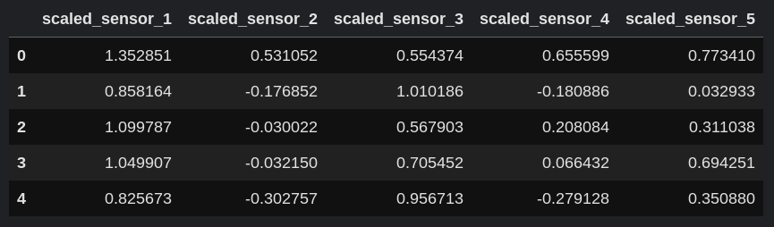
df_scaled = pd.DataFrame(scaler.fit_transform(df[sensor_cols].to_numpy()), columns=scaled_cols)
df_scaled.head()
Next, let's combine the scaled dataframe with the original dataframe using pd.concat.
df = pd.concat([df, df_scaled], axis=1)
Determining Feature Importance Using Mutual Information
Now that we have created several new features, we can test whether they have any relationship with the target variables to determine which features to train the model on and which ones to discard.
First, let's create two variables: X, which stores the features, and y, which stores the labels.
To create X, we'll first create a list of the columns we want to keep.
all_features = list(df.columns)
print(all_features)
['date_time', 'deg_C', 'relative_humidity', 'absolute_humidity', 'sensor_1', 'sensor_2', 'sensor_3', 'sensor_4', 'sensor_5', 'target_carbon_monoxide', 'target_benzene', 'target_nitrogen_oxides', 'temp_plus_humidity', 'temp_minus_humidity', 'temp_times_humidity', 'temp_divided_by_humidity', 'deg_F', 'max_water_vapor', 'date_time_parsed', 'hour', 'day', 'month', 'year', 'quarter', 'binned_sensor_1', 'binned_sensor_2', 'binned_sensor_3', 'binned_sensor_4', 'binned_sensor_5', 'scaled_sensor_1', 'scaled_sensor_2', 'scaled_sensor_3', 'scaled_sensor_4', 'scaled_sensor_5']
We will not include the columns date_time or date_time_parsed as those data types will not be understood by a machine learning model or the mutual information function. We will also exclude the columns target_carbon_monoxide, target_benzene, and target_nitrogen_oxides since they are the labels.
for x in ('date_time', 'date_time_parsed', 'target_carbon_monoxide', 'target_benzene', 'target_nitrogen_oxides'):
    all_features.remove(x)
Now, let's create a variable X that stores all the features:
X = df[all_features]
Let's also create a variable y that stores all the labels:
y = df[["target_carbon_monoxide", "target_benzene", "target_nitrogen_oxides"]]
Scikit-learn provides a function called mutual_info_regression. We will create a function that returns the mutual information between each feature and a given label. We will then call this function once for each label we are trying to predict.
def mi_scores(X, y):
    mi_scores = mutual_info_regression(X, y)
    mi_scores = pd.Series(mi_scores, name="Mutual Information Scores", index=X.columns)
    mi_scores = mi_scores.sort_values(ascending=False)
    return mi_scores
print(mi_scores(X, y["target_carbon_monoxide"]))
print("\n")
print(mi_scores(X, y["target_benzene"]))
print("\n")
print(mi_scores(X, y["target_nitrogen_oxides"]))
scaled_sensor_2             1.041325
sensor_2                    1.039792
scaled_sensor_1             0.743840
sensor_1                    0.743327
sensor_5                    0.685566
scaled_sensor_5             0.685314
scaled_sensor_3             0.615222
sensor_3                    0.614230
binned_sensor_2             0.613156
binned_sensor_1             0.551121
binned_sensor_5             0.507127
sensor_4                    0.387663
scaled_sensor_4             0.387578
binned_sensor_3             0.346512
hour                        0.330685
binned_sensor_4             0.255194
month                       0.086405
temp_divided_by_humidity    0.063835
deg_C                       0.049258
deg_F                       0.047152
absolute_humidity           0.046896
temp_minus_humidity         0.043112
relative_humidity           0.041701
quarter                     0.038334
max_water_vapor             0.036603
temp_plus_humidity          0.034266
day                         0.021176
temp_times_humidity         0.017850
year                        0.000000
Name: Mutual Information Scores, dtype: float64


scaled_sensor_2             1.998963
sensor_2                    1.997717
binned_sensor_2             0.940828
sensor_3                    0.907664
scaled_sensor_3             0.907587
scaled_sensor_5             0.834486
sensor_5                    0.834000
sensor_1                    0.780820
scaled_sensor_1             0.780512
scaled_sensor_4             0.669859
sensor_4                    0.669768
binned_sensor_5             0.600453
binned_sensor_3             0.562740
binned_sensor_1             0.552489
binned_sensor_4             0.456760
hour                        0.323144
max_water_vapor             0.197541
absolute_humidity           0.166549
relative_humidity           0.129360
temp_divided_by_humidity    0.128394
temp_minus_humidity         0.124984
deg_F                       0.117952
deg_C                       0.115604
temp_plus_humidity          0.092767
month                       0.085944
day                         0.052050
temp_times_humidity         0.050124
quarter                     0.021046
year                        0.016426
Name: Mutual Information Scores, dtype: float64


scaled_sensor_2             0.552424
sensor_2                    0.552320
sensor_5                    0.529137
scaled_sensor_5             0.529062
scaled_sensor_3             0.486574
sensor_3                    0.486535
binned_sensor_5             0.417100
scaled_sensor_1             0.375028
sensor_1                    0.374858
binned_sensor_2             0.366994
binned_sensor_1             0.308272
binned_sensor_3             0.284557
month                       0.277641
hour                        0.195761
scaled_sensor_4             0.190657
sensor_4                    0.190559
quarter                     0.188732
binned_sensor_4             0.121445
temp_minus_humidity         0.062636
absolute_humidity           0.061017
max_water_vapor             0.050784
temp_divided_by_humidity    0.048532
deg_F                       0.047627
deg_C                       0.044749
day                         0.043873
temp_plus_humidity          0.042214
temp_times_humidity         0.038651
relative_humidity           0.025827
year                        0.003576
Name: Mutual Information Scores, dtype: float64
There is no specific score that tells us whether a feature is important or not, but we have determined the order of the most important features.
We can see that the sensors all have the highest mutual information scores, and some date/time features also have relatively high scores. Based on this information, we will keep all the sensor features (including the binned and scaled ones) as well as the month, hour, and quarter features.
to_keep = ["month", "hour", "quarter"]
for i in range(5):
    to_keep.append(f"sensor_{i+1}")
    to_keep.append(f"binned_sensor_{i+1}")
    to_keep.append(f"scaled_sensor_{i+1}")
print(to_keep)
['month', 'hour', 'quarter', 'sensor_1', 'binned_sensor_1', 'scaled_sensor_1', 'sensor_2', 'binned_sensor_2', 'scaled_sensor_2', 'sensor_3', 'binned_sensor_3', 'scaled_sensor_3', 'sensor_4', 'binned_sensor_4', 'scaled_sensor_4', 'sensor_5', 'binned_sensor_5', 'scaled_sensor_5']
Finally, we will include only those features we have decided to keep:
X = X[to_keep]
Testing and Results
We will first create, train, and evaluate a model on the original data, and we will compare it to the performance of the model that is trained on the feature engineered data.
Training on the Original Data
First, let's load the original data:
original_df = pd.read_csv("train.csv")
Let's separate into original_X and original_y
columns = list(original_df.columns)
for col in ("date_time", "target_nitrogen_oxides", "target_benzene", "target_carbon_monoxide"):
    columns.remove(col)
original_X = original_df[columns]
original_y = original_df[["target_nitrogen_oxides", "target_benzene", "target_carbon_monoxide"]]
Let's split the data into 80% training and 20% testing (we won't shuffle so that we can use the same samples for the other model):
X_train, X_test, y_train, y_test = train_test_split(original_X, original_y, test_size=0.2, shuffle=False)
Finally, we will create a model for each target variable and output its mean squared error.
for label in ("target_nitrogen_oxides", "target_benzene", "target_carbon_monoxide"):
    rf = RandomForestRegressor(n_estimators=500)
    rf.fit(X_train, y_train[label])
    preds = rf.predict(X_test)
    print(label + ": " + str(mean_squared_error(preds, y_test[label])))
target_nitrogen_oxides: 55648.86831157129
target_benzene: 2.2838145447083664
target_carbon_monoxide: 1.0311513765846796
Testing on the Feature Engineered Data
We have already created variables X and y for the feature engineered data. The next step is to split the data into 80% training and 20% testing:
X_train, X_test, y_train, y_test = train_test_split(X, y, test_size=0.2, shuffle=False)
The code to train and test the models remains the same:
for label in ("target_nitrogen_oxides", "target_benzene", "target_carbon_monoxide"):
    rf = RandomForestRegressor(n_estimators=500)
    rf.fit(X_train, y_train[label])
    preds = rf.predict(X_test)
    print(label + ": " + str(mean_squared_error(preds, y_test[label])))
target_nitrogen_oxides: 47670.98778886509
target_benzene: 2.2403446973998626
target_carbon_monoxide: 0.9799029642445529
As we can see, the model performs better on the feature engineered data than it does on the original data.
Conclusion
In this article at OpenGenus, we saw different feature engineering techniques and how they can be applied to enhance model performance. Feature engineering is a trial-and-error process, so further experimenting with what features to create or remove can lead to potentially even better results.
That's it for this article, and thank you for reading!
References
- Holbrook, R. (n.d.). Mutual Information. Kaggle. https://www.kaggle.com/code/ryanholbrook/mutual-information/tutorial
- Kaggle. (2021, July 1). Tabular Playground Series - Jul 2021 | Kaggle [Dataset]. https://www.kaggle.com/competitions/tabular-playground-series-jul-2021/data?select=train.csv