
Our company strategically invests in customers through various means such as acquisition costs, offline ads, promotions, and discounts to drive revenue and ensure profitability. These actions naturally lead to some customers becoming highly valuable in terms of their lifetime value. However, we also encounter customers whose behavior negatively impacts our profitability. It is crucial for us to identify these patterns of behavior, segment customers accordingly, and take appropriate actions.
The process of calculating the Lifetime Value is relatively straightforward. First, we need to determine a specific time window, which can range from 3 to 24 months. By applying the following equation, we can compute the Lifetime Value for each customer within that particular time frame:
Lifetime Value = Total Gross Revenue - Total Cost
This equation provides us with the historical lifetime value. If we observe some customers with significantly high negative lifetime values historically, it may indicate that corrective actions should have been taken earlier.
To address this challenge, we are embarking on building a simple machine learning model that can accurately predict the lifetime value of our customers.
Key Steps for Lifetime Value Prediction:
-
Define an Appropriate Time Frame for Customer Lifetime Value Calculation:
The time frame selection depends on the industry, business model, and other factors. In our case, we have chosen a 6-month time frame as a suitable period. -
Identify the Features for Prediction:
The RFM (Recency, Frequency, Monetary) scores for each customer ID, which we previously calculated, serve as ideal features for our prediction model. To implement this effectively, we will split our dataset into two parts. We will utilize three months of data to calculate RFM scores, and then use these scores to predict the customer's behavior over the next 6 months. Therefore, we need to create two dataframes and append RFM scores to them.
Following these initial steps, we can seamlessly calculate Customer Lifetime Value (CLTV) and proceed to train and test our machine learning model to assess its usefulness in predicting customer lifetime values.
Content:
- Dataset
- Importing necessary libraries
- Feature Engineering
- Segmentation Techniques
- Calculating recency
- Assigning a recency score
- Cluster ordering
- Calculating Frequency
- Frequency clusters
- Calculating Revenue
- Revenue clusters
- Overall scores based on RFM clustering
- Calculate Customer Lifetime Value
- Model for Customer Lifetime Value Prediction
- Conclusion
Dataset:
The dataset titled "Customer Segmentation" available on Kaggle, provided by user sergeymedvedev, is a collection of customer data designed for the purpose of customer segmentation. Customer segmentation is a vital technique in marketing and data analysis, where customers are grouped into distinct segments based on specific characteristics and behaviors. This helps businesses better understand their customer base, tailor marketing strategies, and improve customer satisfaction.
The dataset contains various attributes related to customer behavior, demographics, and purchase history. It includes the following key features:
- CustomerID: A unique identifier for each customer.
- InvoiceNo: The identification number of the invoice associated with a particular transaction.
- InvoiceDate: The date and time when the transaction occurred.
- Quantity: The quantity of items purchased in each transaction.
- UnitPrice: The unit price of each item purchased.
- Country: The country where the customer resides.
The dataset seems to be related to retail or e-commerce, as it contains information typically found in transactional data. The provided data allows for exploring customer purchasing patterns, analyzing customer preferences, and understanding which products are more popular among specific segments of customers.
The primary goal of using this dataset is likely to conduct customer segmentation analyses to group customers into distinct clusters based on their purchasing behavior, geographical location, or other relevant characteristics. Businesses can use the resulting segments to target different customer groups with personalized marketing campaigns, optimize inventory management, and improve overall customer experience.
Before conducting any analysis, data cleaning and preprocessing may be necessary to handle missing values, outliers, or inconsistencies in the data. Additionally, further feature engineering might be required to extract additional insights from the dataset.
Access the dataset from here1. Importing necessary libraries
from __future__ import division
from datetime import datetime, timedelta,date
import pandas as pd
%matplotlib inline
from sklearn.metrics import classification_report,confusion_matrix
import matplotlib.pyplot as plt
import numpy as np
import seaborn as sns
from sklearn.cluster import KMeans
import plotly as py
import plotly.offline as pyoff
import plotly.graph_objs as go
import xgboost as xgb
from sklearn.model_selection import KFold, cross_val_score, train_test_split
import xgboost as xgb
Import the dataset:
df=pd.read_csv('/content/customer_segmentation.csv', encoding='cp1252')
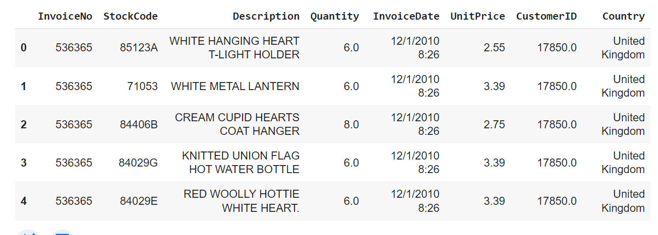
Print the first five data points of the dataset:
#initate plotly
pyoff.init_notebook_mode()
df.head()
Out:
2. Feature Engineering
# converting the type of Invoice Date Field from string to datetime.
df['InvoiceDate'] = pd.to_datetime(df['InvoiceDate'])

# creating YearMonth field for the ease of reporting and visualization
df['InvoiceYearMonth'] = df['InvoiceDate'].map(lambda date: 100*date.year + date.month)
# get statistical inference of the dataset
df.describe()
Out: 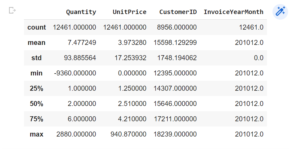
get the number of non null values for each country's records
df['Country'].value_counts()
Out: 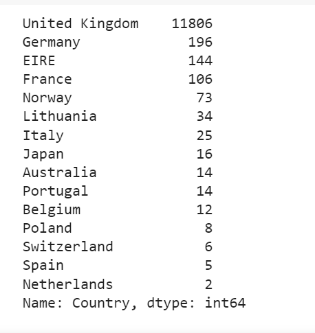
Starting from this part, we will be focusing on UK data only (which has the most records). We can get the monthly active customers by counting unique CustomerIDs. The same analysis can be carried out for customers of other countries as well.
# we will be using only UK data
df_uk = df.query("Country=='United Kingdom'").reset_index(drop=True)
Segmentation Techniques
There are various segmentation methods that can be employed based on specific objectives. For instance, if the aim is to enhance customer retention, one can perform a segmentation based on churn probability and implement appropriate strategies. However, there are several common and valuable segmentation techniques available. In this instance, we will adopt one of these techniques for our business: RFM (Recency - Frequency - Monetary Value) segmentation.
Theoretically, after applying the RFM segmentation, we will categorize customers into the following groups:
-
Low Value: This group comprises customers who are less active compared to others, infrequent buyers or visitors, and generate minimal to no revenue, possibly even causing negative revenue.
-
Mid Value: Customers falling into this category are moderately engaged with our platform. While they are not as active as the High-Value group, they are relatively frequent users and generate moderate revenue.
-
High Value: This is the most desirable group that we aim to retain. These customers exhibit high revenue generation, frequent engagement, and low inactivity.
To implement this methodology, we need to calculate the Recency, Frequency, and Monetary Value (referred to as Revenue) for each customer. By applying unsupervised machine learning techniques, we can then identify different groups or clusters for each segment. This process is known as RFM Clustering.
Let's proceed with the coding phase to perform the RFM Clustering and observe the outcomes of our segmentation.
3. Calculating recency
"Recency" refers to the measure of how recently a customer made a purchase or engaged with the platform. It helps us understand the level of activity and engagement of each customer based on the time elapsed since their last interaction. Customers who made recent purchases or had recent engagement will have lower recency scores, indicating higher activity, while customers who have been inactive for an extended period will have higher recency scores, suggesting lower activity or potential churn. By clustering customers based on their recency scores, we can identify different segments and tailor our strategies accordingly.
To determine the recency score, we must identify the most recent purchase date for each customer and calculate the number of days they have been inactive since that purchase. Once we have the count of inactive days for each customer, we will utilize K-means* clustering to assign the customers their respective recency scores.
Now, let's proceed with the calculation of the recency scores.
# create a generic user dataframe to keep CustomerID and new segmentation scores
df_user = pd.DataFrame(df['CustomerID'].unique())
df_user.columns = ['CustomerID']
df_user.head()
Out: 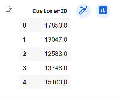
df_uk.head()
Out: 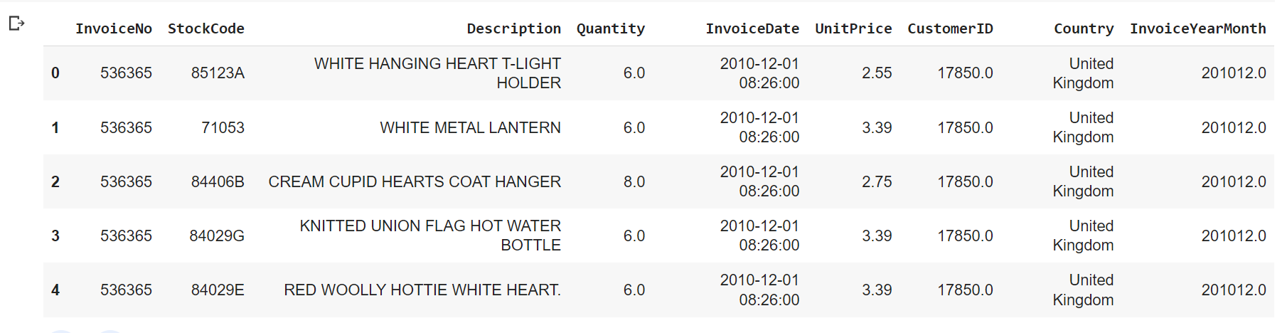
# get the max purchase date for each customer and create a dataframe with it
df_mxp = df_uk.groupby('CustomerID').InvoiceDate.max().reset_index()
df_mxp.columns = ['CustomerID','MaxPurchaseDate']
# Compare the last transaction of the dataset with last transaction dates of the individual customer IDs.
df_mxp['Recency'] = (df_mxp['MaxPurchaseDate'].max() - df_mxp['MaxPurchaseDate']).dt.days
# merge this dataframe to our new user dataframe
df_user = pd.merge(df_user, df_mxp[['CustomerID','Recency']], on='CustomerID')
# print head of df_user
df_user.head()
Out: 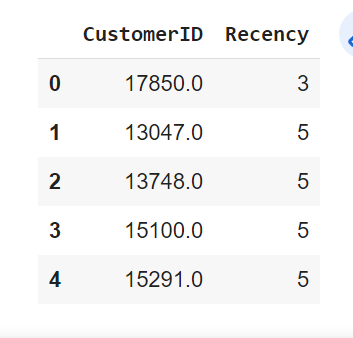
Assigning a recency score
Utilizing K-means clustering to assign a recency score is a powerful approach in customer segmentation, but determining the optimal number of clusters for the K-means algorithm is a critical step in the process. To address this challenge, we will employ the "Elbow Method," a widely used technique that aids in identifying the optimal number of clusters based on the concept of inertia.
Inertia, also known as within-cluster sum of squares, measures how closely related data points within a cluster are to its centroid. The goal of K-means clustering is to minimize the inertia, as this ensures that the clusters formed are compact and well-separated. However, we need to find the sweet spot where adding more clusters doesn't significantly reduce inertia, leading to diminishing returns.
The Elbow Method involves plotting the inertia against different values of the number of clusters. As the number of clusters increases, the inertia typically decreases, as each cluster tends to have fewer data points, resulting in tighter clusters. However, there is a point where the rate of inertia reduction starts to level off. This point is akin to the "elbow" in the inertia graph, and it represents the optimal number of clusters for the given dataset.
To apply the Elbow Method, we will evaluate the inertia for different cluster numbers and observe the graph. As the number of clusters increases, the inertia will decrease, and the graph will exhibit a downward trend. The point where the inertia starts to level off, forming an elbow shape, indicates the optimal cluster number. This number represents the ideal balance between minimizing inertia and preventing an excessive increase in the number of clusters, ensuring meaningful and interpretable segments.
Let's dive into the code snippet to implement the Elbow Method and visualize the inertia graph. By doing so, we can confidently determine the most suitable number of clusters for our K-means clustering algorithm, leading us towards more effective customer segmentation and personalized marketing strategies.
from sklearn.cluster import KMeans
dict={} # error
df_rec = df_user[['Recency']]
for k in range(1, 10):
    kmeans = KMeans(n_clusters=k, max_iter=1000).fit(df_rec)
    df_rec["clusters"] = kmeans.labels_  #cluster names corresponding to recency values
    dict[k] = kmeans.inertia_ #dict corresponding to clusters
plt.figure()
plt.plot(list(dict.keys()), list(dict.values()))
plt.xlabel("Number of cluster")
plt.show()
Out: 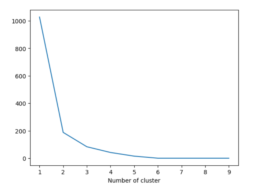
Here it looks like 3 is the optimal one. Based on business requirements, we can go ahead with less or more clusters. We will be selecting 4 for this example
# build 4 clusters for recency and add it to dataframe
kmeans = KMeans(n_clusters=4)
df_user['RecencyCluster'] = kmeans.fit_predict(df_user[['Recency']])
Cluster ordering
In our pursuit of optimizing customer segmentation, we often encounter the need to order clusters in a way that enables us to effectively target specific customer groups with tailored marketing strategies. The provided code snippet demonstrates a valuable function called order_cluster, which facilitates the ordering of clusters based on certain criteria, such as 'Recency' in this case.
The function takes several parameters, including 'cluster_field_name' (the field representing cluster labels), 'target_field_name' (the field on which the clusters will be ordered), 'df' (the DataFrame containing the data), and 'ascending' (a boolean value indicating the desired sorting order). The ultimate objective is to rearrange the clusters based on their average 'Recency' values to facilitate better decision-making and customer engagement.
Here's a step-by-step explanation of the order_cluster function:
-
Creation of a New DataFrame for Cluster Averages:
First, the function groups the DataFrame 'df' by the 'RecencyCluster' field (representing cluster labels) and calculates the mean 'Recency' value for each cluster. The results are stored in a new DataFrame called 'df_new.' -
Sorting Clusters based on Averages:
Next, the function sorts the clusters in 'df_new' based on their average 'Recency' values, either in ascending or descending order, as specified by the 'ascending' parameter. This step allows us to identify clusters with the highest or lowest 'Recency,' depending on the intended sorting order. -
Assigning New Cluster Indices:
To preserve the cluster ordering, 'df_new' is updated with a new index, which reflects the new order of clusters after sorting. This index information will be utilized to reorder the original DataFrame 'df.' -
Merging and Finalizing Cluster Ordering:
The function then merges the original DataFrame 'df' with the updated 'df_new,' matching the 'RecencyCluster' field to align the clusters correctly. The original 'RecencyCluster' field is dropped, and the new index is renamed as 'RecencyCluster' to finalize the ordering of the clusters.
In the provided example, the order_cluster function is applied to the 'df_user' DataFrame, ordering the 'RecencyCluster' based on the average 'Recency' values in descending order (largest to smallest). This reordering enhances the segmentation, allowing us to identify clusters with higher recency (less recent activity) for targeted engagement.
By employing this cluster ordering technique, businesses can effectively prioritize and address customer segments based on specific attributes, leading to more personalized marketing initiatives, improved customer retention, and overall business growth.
# function for ordering cluster numbers
def order_cluster(cluster_field_name, target_field_name,df,ascending):
    new_cluster_field_name = 'new_' + cluster_field_name
    df_new = df.groupby(cluster_field_name)[target_field_name].mean().reset_index()
    df_new = df_new.sort_values(by=target_field_name,ascending=ascending).reset_index(drop=True)
    df_new['index'] = df_new.index
    df_final = pd.merge(df,df_new[[cluster_field_name,'index']], on=cluster_field_name)
    df_final = df_final.drop([cluster_field_name],axis=1)
    df_final = df_final.rename(columns={"index":cluster_field_name})
    return df_final

df_user = order_cluster('RecencyCluster', 'Recency',df_user,False)
4. Calculating Frequency
In customer segmentation analysis, the concept of "Frequency" plays a crucial role in understanding customer transaction patterns and their engagement with a business. Frequency refers to the number of times a customer has placed orders or engaged in transactions over a specific period. By analyzing frequency, businesses gain valuable insights into customer loyalty, activity levels, and overall engagement with the company's products or services.
To create frequency clusters, we start by calculating the total number of orders for each customer. This process involves counting how many times each customer has made a purchase or conducted a transaction. The resulting frequency values represent the number of interactions a customer has had with the business within the defined time frame.
Once we obtain the frequency values for all customers, we can begin to explore the distribution and patterns within our customer database. By visualizing frequency data, we can identify common transaction behaviors, such as whether the majority of customers engage with the business frequently or if there is a more dispersed distribution with varying levels of activity.
Understanding customer frequency patterns is crucial for several reasons:
-
Identifying High-Frequency Customers: Customers with a high frequency of transactions are often more loyal and engaged with the brand. These valuable customers can become a focus for retention strategies and targeted marketing campaigns.
-
Segmenting Customers Based on Engagement: By clustering customers into different frequency segments, businesses can create tailored marketing strategies for each segment. For instance, frequent buyers may receive loyalty rewards, while less active customers may receive incentives to re-engage.
-
Detecting Churn or Inactivity: Low-frequency or inactive customers may indicate potential churn or disengagement. Identifying these customers allows businesses to implement strategies to re-engage them and prevent attrition.
The calculated frequency values enable businesses to better understand customer preferences, behavior, and loyalty. Armed with this knowledge, companies can optimize marketing efforts, improve customer retention, and enhance overall customer satisfaction.
# get order counts for each user and create a dataframe with it
df_freq = df_uk.groupby('CustomerID').InvoiceDate.count().reset_index()
df_freq.columns = ['CustomerID','Frequency']
# add this data to our main dataframe
df_user = pd.merge(df_user, df_freq, on='CustomerID')
df_user.head()
Out: 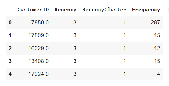
Frequency clusters
Just like recency score we will apply elbow method to obtain frequency clusters
from sklearn.cluster import KMeans
dict={} # error
df_rec = df_user[['Frequency']]
for k in range(1, 10):
    kmeans = KMeans(n_clusters=k, max_iter=1000).fit(df_rec)
    df_rec["clusters"] = kmeans.labels_  #cluster names corresponding to recency values
    dict[k] = kmeans.inertia_ #dict corresponding to clusters
plt.figure()
plt.plot(list(dict.keys()), list(dict.values()))
plt.xlabel("Number of cluster")
plt.show()
Out: 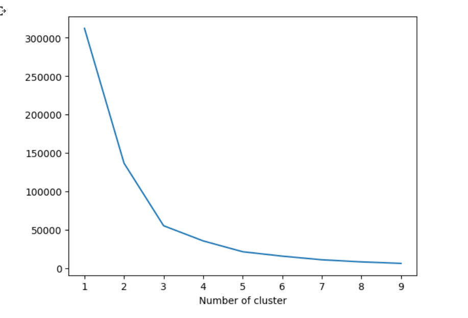
By Elbow method, clusters number should be 4 as after 4, the graph goes down.
# Applying k-Means
kmeans=KMeans(n_clusters=4)
df_user['FrequencyCluster']=kmeans.fit_predict(df_user[['Frequency']])

#order the frequency cluster
df_user = order_cluster('FrequencyCluster', 'Frequency', df_user, True )
5. Calculating Revenue
Revenue stands as a critical metric that sheds light on customer spending patterns and the financial impact of their interactions with a business. Revenue represents the total amount of money generated from customer transactions or purchases over a specific period. By analyzing revenue, businesses gain valuable insights into the financial performance of their customer base and can make informed decisions to optimize their sales strategies and overall profitability.
To explore customer spending behaviors and their financial contributions, we first calculate the revenue associated with each customer. This involves aggregating the total monetary value of all transactions made by a customer within the specified time frame. The resulting revenue values demonstrate the extent to which each customer contributes to the company's overall financial success.
Once we have obtained the revenue values for each customer, we can further examine the distribution and patterns within our customer database. By visualizing revenue data, such as through a histogram, we can discern common spending behaviors among customers. This could reveal whether the majority of customers make small, moderate, or substantial purchases and how this impacts the overall revenue landscape.
Understanding revenue patterns is instrumental for several crucial business strategies:
-
Identifying High-Value Customers: Customers with significant revenue contributions are typically considered high-value customers. Recognizing these customers allows businesses to prioritize their needs, implement personalized marketing, and cultivate strong customer loyalty.
-
Segmenting Customers Based on Spending: Clustering customers into different revenue segments allows businesses to create targeted marketing campaigns tailored to each group's spending behavior. High-spenders may receive exclusive offers, while moderate spenders could receive incentives to boost their spending.
-
Analyzing Revenue Growth and Trends: Monitoring revenue trends over time helps businesses evaluate their financial performance and identify growth opportunities. By comparing revenue data across different periods, businesses can identify seasonal trends and adjust their strategies accordingly.
Revenue is an essential metric that goes hand-in-hand with other customer-related data, such as frequency and recency, to form a comprehensive understanding of customer behavior. Armed with this knowledge, businesses can optimize their sales and marketing efforts, maximize customer lifetime value, and foster strong customer relationships.
#calculate revenue for each customer
df_uk['Revenue'] = df_uk['UnitPrice'] * df_uk['Quantity']
df_rev = df_uk.groupby('CustomerID').Revenue.sum().reset_index()
df_rev.head()
Out: 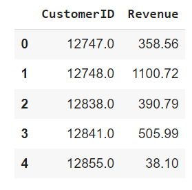
#merge it with our main dataframe
df_user = pd.merge(df_user, df_rev, on='CustomerID')
Revenue clusters
Just like recency score and frequency we will apply elbow method to obtain revenue clusters
from sklearn.cluster import KMeans
dict={} # error
df_rec = df_user[['Revenue']]
for k in range(1, 10):
    kmeans = KMeans(n_clusters=k, max_iter=1000).fit(df_rec)
    df_rec["clusters"] = kmeans.labels_  #cluster names corresponding to recency values
    dict[k] = kmeans.inertia_ #dict corresponding to clusters
plt.figure()
plt.plot(list(dict.keys()), list(dict.values()))
plt.xlabel("Number of cluster")
plt.show()
Out: 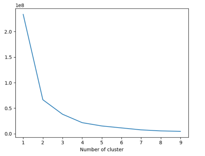
From elbow's method, we find that clusters can be 3 or 4. Lets take 4 as the number of clusters
#apply clustering
kmeans = KMeans(n_clusters=4)
df_user['RevenueCluster'] = kmeans.fit_predict(df_user[['Revenue']])
#order the cluster numbers
df_user = order_cluster('RevenueCluster', 'Revenue',df_user,True)
6. Overall scores based on RFM clustering
We have scores (cluster numbers) for recency, frequency & revenue.
Now we'll create an overall score from these three.
#calculate overall score and use mean() to see details
df_user['OverallScore'] = df_user['RecencyCluster'] + df_user['FrequencyCluster'] + df_user['RevenueCluster']
df_user.groupby('OverallScore')['Recency','Frequency','Revenue'].mean()
Out: 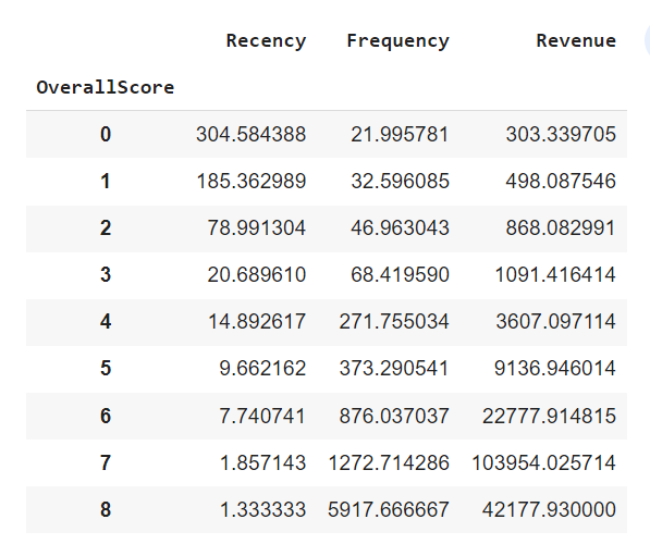
Score 0 is our worst customer and score 8 is the best customer.
df_user['Segment'] = 'Low-Value'
df_user.loc[df_user['OverallScore']>2,'Segment'] = 'Mid-Value'
df_user.loc[df_user['OverallScore']>4,'Segment'] = 'High-Value'
df_user
Out: 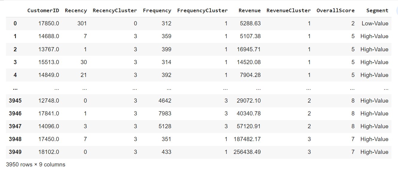
7. Calculate Customer Lifetime Value
With our feature set prepared and ready for analysis, the next crucial step in our journey towards effective customer segmentation and personalized marketing is to calculate the 6-month Customer Lifetime Value (LTV) for each customer. The LTV represents the total value generated from customer transactions over a specific period, indicating the monetary impact of their interactions with our business.
The formula to calculate LTV is relatively straightforward:
LTV = Total Gross Revenue - Total Cost
However, it's worth noting that the dataset we are working with does not specify any cost information. As a result, we can directly consider the "Revenue" as the LTV in this context. The "Revenue" becomes a key metric representing the overall financial value generated by each customer over the 6-month period.
df_uk['InvoiceDate'].describe()
Out: 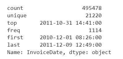
We observe customer activity starting from December 1, 2010. To ensure we focus on established customers, we will only consider those who have been with us since March onwards. From this group of customers, we will create two distinct subgroups based on the timeframe of analysis: one group will be evaluated over a 3-month period, while the other will be assessed over a 6-month period.
# Convert date objects to datetime64[ns]
date_3m_start = pd.to_datetime(datetime(2011, 3, 1))
date_3m_end = pd.to_datetime(datetime(2011, 6, 1))
date_6m_start = pd.to_datetime(datetime(2011, 6, 1))
date_6m_end = pd.to_datetime(datetime(2011, 12, 1))

df_3m = df_uk[(df_uk['InvoiceDate'] < date_3m_end) & (df_uk['InvoiceDate'] >= date_3m_start)].reset_index(drop=True)  # Transactions within a 3-month period
df_6m = df_uk[(df_uk['InvoiceDate'] >= date_6m_start) & (df_uk['InvoiceDate'] < date_6m_end)].reset_index(drop=True)  # Transactions within a 6-month period
#calculate revenue and create a new dataframe for it
df_6m['Revenue'] = df_6m['UnitPrice'] * df_6m['Quantity']
df_user_6m = df_6m.groupby('CustomerID')['Revenue'].sum().reset_index()
df_user_6m.columns = ['CustomerID','m6_Revenue']
df_user_6m.head()
Out: 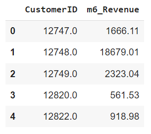
import plotly.graph_objects as go
import plotly.offline as pyoff

# Plot LTV histogram
plot_data = [
    go.Histogram(
        x=df_user_6m['m6_Revenue']
    )
]

plot_layout = go.Layout(
        title='6m Revenue'
    )

fig = go.Figure(data=plot_data, layout=plot_layout)
pyoff.iplot(fig)
Out: 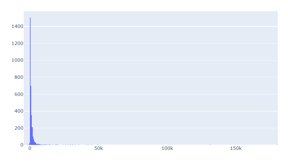
The histogram provides a clear representation that we have customers with negative Customer Lifetime Value (LTV), and there are also some outliers in the data. To ensure the development of a robust machine learning model, it is logical to filter out these outliers.
Moving forward, the next step involves merging our 3-month data with 'tx_uk' and similarly, merging the 6-month dataframe with 'tx_uk'. This merging process will allow us to explore the correlations between the LTV and the set of features we have obtained for the customers. By establishing these correlations, we can gain valuable insights into how different features influence the LTV and potentially uncover meaningful patterns that can aid in building an effective machine learning model.
df_merge = pd.merge(df_user, df_user_6m, on='CustomerID', how='left') #Only people who are in the timeline of df_user_6m
df_merge = df_merge.fillna(0)
plotting the histogram,
df_graph = df_merge.query("m6_Revenue < 50000") #because max values are ending at 50,000 as seen in graph above

plot_data = [
    go.Scatter(
        x=df_graph.query("Segment == 'Low-Value'")['OverallScore'],
        y=df_graph.query("Segment == 'Low-Value'")['m6_Revenue'],
        mode='markers',
        name='Low',
        marker= dict(size= 7,
            line= dict(width=1),
            color= 'blue',
            opacity= 0.8
           )
    ),
        go.Scatter(
        x=df_graph.query("Segment == 'Mid-Value'")['OverallScore'],
        y=df_graph.query("Segment == 'Mid-Value'")['m6_Revenue'],
        mode='markers',
        name='Mid',
        marker= dict(size= 9,
            line= dict(width=1),
            color= 'green',
            opacity= 0.5
           )
    ),
        go.Scatter(
        x=df_graph.query("Segment == 'High-Value'")['OverallScore'],
        y=df_graph.query("Segment == 'High-Value'")['m6_Revenue'],
        mode='markers',
        name='High',
        marker= dict(size= 11,
            line= dict(width=1),
            color= 'red',
            opacity= 0.9
           )
    ),
]

plot_layout = go.Layout(
        yaxis= {'title': "6m LTV"},
        xaxis= {'title': "RFM Score"},
        title='LTV'
    )
fig = go.Figure(data=plot_data, layout=plot_layout)
pyoff.iplot(fig)
Out: 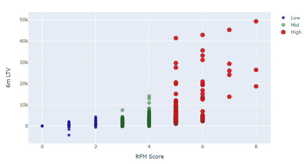
The correlation between the overall RFM score and revenue is evident from the visualization, showing a positive relationship. Customers with higher RFM scores tend to have higher Customer Lifetime Value (LTV).
Before proceeding with the machine learning model, we must determine the type of machine learning problem at hand. LTV itself represents a regression problem, where a machine learning model can predict the monetary value of the LTV. However, for our specific case, we aim to group customers into LTV segments, making it more actionable and easier to communicate with others. By employing K-means clustering, we can identify existing LTV groups and create segments based on this information.
Taking into account the business aspect of this analysis, it is essential to treat customers differently based on their predicted LTV. For this particular example, we will utilize clustering to form three segments (although the actual number of segments can vary depending on specific business dynamics and objectives):
- Low LTV
- Mid LTV
- High LTV
Applying the K-means clustering technique will enable us to make informed decisions based on the distinct characteristics of each segment, tailoring marketing strategies and customer engagement accordingly. By grouping customers into these segments, businesses can maximize their efficiency and effectiveness in catering to different customer needs and preferences.
Let's proceed with the implementation of K-means clustering to define these segments and observe their distinctive characteristics. This step will lay the foundation for more targeted and personalized customer management, ultimately leading to enhanced customer satisfaction and business success.
#remove outliers
df_merge = df_merge[df_merge['m6_Revenue']<df_merge['m6_Revenue'].quantile(0.99)]

#creating 3 clusters
kmeans = KMeans(n_clusters=3)
df_merge['LTVCluster'] = kmeans.fit_predict(df_merge[['m6_Revenue']])

df_merge.head()
Out: 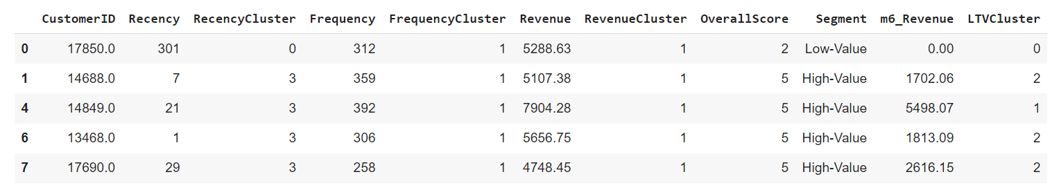
#order cluster number based on LTV
df_merge = order_cluster('LTVCluster', 'm6_Revenue',df_merge,True)

#creatinga new cluster dataframe
df_cluster = df_merge.copy()

#see details of the clusters
df_cluster.groupby('LTVCluster')['m6_Revenue'].describe()
Out: 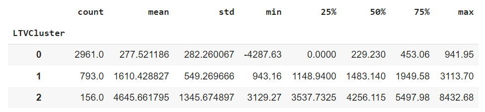
The LTV clustering process is now complete, and the distinctive characteristics of each cluster are outlined above.
Cluster 2 emerges as the most favorable segment, boasting an average LTV of 8.2k, while Cluster 0 represents the least favorable, with an average LTV of 396.
Before proceeding with training the machine learning model, several crucial steps need to be undertaken:
-
Feature Engineering: This step involves refining and transforming the existing features to extract relevant information and enhance the predictive power of the model.
-
Conversion of Categorical Columns to Numerical: To make the data suitable for machine learning algorithms, categorical columns need to be converted into numerical representation.
-
Correlation Analysis of Features with LTV Clusters: We will assess the correlations between the features and our target label, LTV clusters, to identify which features significantly influence the cluster assignments.
-
Splitting Feature Set and Label (LTV): The feature set, denoted as X, and the target label (LTV clusters), denoted as y, will be separated to prepare for the machine learning process. We will use X to predict y, the LTV cluster.
-
Creation of Training and Test Datasets: The dataset will be divided into a Training set, which will be utilized to build the machine learning model, and a Test set, which will serve to evaluate the model's real-world performance.
By following these essential steps, we ensure that our machine learning model is well-prepared, effectively incorporating relevant features, and capable of accurately predicting the LTV clusters. The Test set will enable us to assess the model's generalization to new data, gauging its performance in real-life scenarios. This process sets the stage for making informed decisions, implementing targeted marketing strategies, and ultimately optimizing customer engagement and business success.
df_cluster.head()
Out: 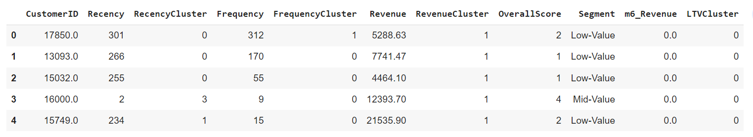
#convert categorical columns to numerical
df_class = pd.get_dummies(df_cluster) #There is only one categorical variable segment

#calculate and show correlations
corr_matrix = df_class.corr()
corr_matrix['LTVCluster'].sort_values(ascending=False)
Out: 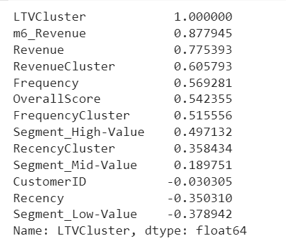
We see that Revenue, Frequency and RFM scores will be helpful for our machine learning models from the correlation with LTVCluster.
#create X and y, X will be feature set and y is the label - LTV
X = df_class.drop(['LTVCluster','m6_Revenue'],axis=1)
y = df_class['LTVCluster']

#split training and test sets
X_train, X_test, y_train, y_test = train_test_split(X, y, test_size=0.05, random_state=56)
8. Model for Customer Lifetime Value Prediction
Given that our LTV clusters consist of three distinct types, we will engage in a multi-class classification approach.
#XGBoost Multiclassification Model
ltv_xgb_model = xgb.XGBClassifier(max_depth=5, learning_rate=0.1,n_jobs=-1).fit(X_train, y_train)

print('Accuracy of XGB classifier on training set: {:.2f}'
       .format(ltv_xgb_model.score(X_train, y_train)))
print('Accuracy of XGB classifier on test set: {:.2f}'
       .format(ltv_xgb_model.score(X_test[X_train.columns], y_test)))

y_pred = ltv_xgb_model.predict(X_test)
Out:
Accuracy of XGB classifier on training set: 0.95
Accuracy of XGB classifier on test set: 0.92
Let's check precision, recall and f-score.
print(classification_report(y_test, y_pred))
Out: 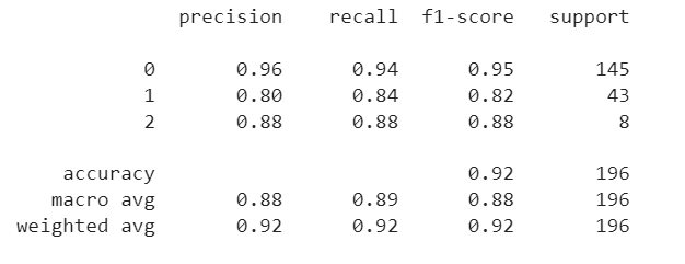
Concluding
After completing the clustering process for Customer Lifetime Value (LTV), we have obtained three distinct clusters:
-
Cluster 0: This cluster exhibits good precision, recall, F1-score, and support. The model accurately identifies 93 out of 100 customers belonging to this cluster (precision) and successfully detects 95% of the actual Cluster 0 customers (recall).
-
Cluster 1: This cluster requires improvement in precision, recall, and F1-score. The model's performance in identifying customers in this cluster needs enhancement.
-
Cluster 2: This cluster has low precision, and the F1-score also needs improvement. The model's accuracy in identifying customers in this cluster needs attention.
To achieve better overall model performance, there are several possible actions that can be taken:
-
Adding More Features and Improving Feature Engineering: By including additional relevant features and refining the existing ones, we can potentially enhance the model's predictive capabilities.
-
Trying Different Models other than XGBoost: Exploring alternative machine learning models can provide insights into which algorithms best suit the specific characteristics of the data and the problem at hand.
-
Applying Hyperparameter Tuning to Current Model: Fine-tuning the hyperparameters of the current XGBoost model can significantly impact its performance, optimizing the model for better results.
-
Adding More Data to the Model: Increasing the size of the dataset, if feasible, can lead to a more comprehensive and robust model, improving its generalization and predictive power.
By implementing these potential improvements, we aim to achieve a more accurate and reliable model for clustering customers based on their LTV, ultimately guiding strategic decision-making, targeted marketing efforts, and customer relationship management.