Sparse matrix multiplication

In this article, we aim to study sparse matrices and the sparse matrix multiplication.

Contents

1. Spase matrix introduction
2. Sparse matrix representations
3. Sparse matrix multiplication
4. Sparse-Sparse matrix multiplication
5. Sparse-Dense matrix multiplication
6. Dense-Sparse matrix product

Sparse matrices

• A Sparse matrix is a matrix in which most of the elements are zero. They commonly appear in scientific applications.
• Sparse matrix multiplication is required to perform the multiplication of two matrixes in less time complexity.
• Most fast matrix multiplication algorithms do not make use of the sparsity of the matrices multiplied.
• So storing all the elements of the matrix is a wastage of memory. Instead only the non-zero elements data in the matrix is to be stored.
• This storage method leads to reduced space requirements and decrease in time of operations performed.
• The number of zero elements divided by the total number of elements is called the sparsity of the matrix.

Sparse matrix representations

• We use a sparse matrix instead of a normal matrix to store only the non-zero element data leading to lesser memory usage. It also leads to faster computations of operations.
• Different reprsentations of data can be used based on the number and distribution of the non-zero elements in the matrix.

Array representation

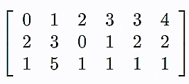
1. The 2D array is used to represent a sparse matrix having three rows.

2. The 'row' row to store the index of the row where the non-zero element is present in the matix.

3. The 'column' row to store the index of the column where the non-zero element is present in the matix.

4. The final row to store the actual value of the non-zero element located at the corresponding row and column position.

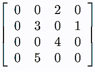
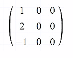
The following is a sparse matrix

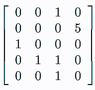
This is the array representation of the above sparse matrix. The last row values are the non-zero elements in the sparse matrix. The first row values and the second row values are the row and column indices of the corresponding final row values in the sparse matrix.

Linked list representation

1. It's easier to insert and delete elements in a linked list compared to an array.
2. Similar to the array representation, this representation requires four fields - row, column, value and the next node.
3. The row field stores the index of the row where the non-zero element is present in the matix.
4. The column field stores the index of the column where the non-zero element is present in the matix.
5. The value field stores the actual value of the non-zero element located at the corresponding row and column position.
6. The next node field stores the reference to the next node.

List of lists

1. Here one list is used to represent the rows in the matrix and each row contains the three fields - column, value and the next node.
2. Column field is used to store columm index of non-zero element, and the value field stores the value of non-zero element, and the next node stores the reference or address to the next node.
3. The elements are sorted by column index for faster lookup and performance.

Dictionary of keys

1. The (row, column) pair of the non-zero element is used as the key and this key maps to the non-zero element.
2. Elements that are not present in the dictionary are considered to be zero.
3. Here sequential access of the elements has poor performance.

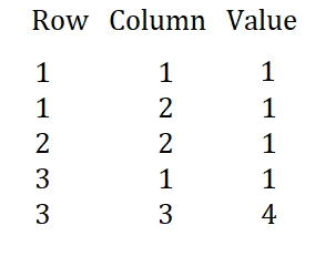
Coordinate fomat (COO)

1. This format uses three subarrays to store the values of non-zero elements and their locations. 2. COO format allows for fast construction of sparse matrices and also conversion to CSR format for fast matrix vector operations. 3. The array 'value' stores the values of the non-zero elements, the 'row' and 'column' arrays store the row index and the column index of the non-zero element values.

Consider the following matrix:

The COO format

Compressed sparse row (CSR)

1. The compressed sparse row format is also called as the Yale format. It represents a matrix using three 1D arrays - value, column index and row index.
2. The value array stores the values of non-zero elements and the column index array stores the column indices of non-zero elements in the matrix.
3. If N is the number of non-zero elements then the value array and the column index arrays are of the length N.
4. The row index array encodes the index in value and column index where a given row starts. An index in the row index array encodes the total number of non-zero elements above this row index.
5. This format is useful since it allows fast row access and matrix multiplications.
6. In the Compressed Sparse Row (CSR) format, the non-zero elements of each row in the sparse matrix are stored in an array continuosly. Another array stores the column index of every non-zero element. Another array stores the starting position of each row of the sparse matrix.

We find the CSR format of the following sparse matrix

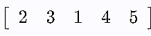
The value array stores the values of the non-zero elements in the matrix.

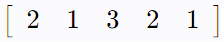
The column index array stores the column indices of the non-zero elements in the matrix.

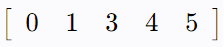
The row index value for a given index 'i' can be found by adding the number of non-zero elements in 'i' row with the previous row index array value.

Compressed sparse column (CSC or CCS)

1. Compressed sparse column is similar to compressed sparse row. Here instead of storing column indices of non-zero elements like in CSR, row indices of non-zero elements are stored in the row index array.
2. The values of non-zero elements are stored in the value array and the column index array stores the list of indices of value array where each column starts in the original matrix.

Sparse matrix multiplication

1. Given two sparse matrices to multiply.
2. Since most elements are zero, to decrease running time complexity and save space we store the non-zero elements only. Various formats can be used- array representation, list of lists, dictionary of keys, CSR, CSC and so on. The resultant matrix of mutliplication can also be stored in this format. This helps to quickly detect zeroes to skip operations that involve multiplications with 0.
3. We first find the transpose of the second matrix. The transpose of a matrix is found by interchanging its rows into columns or columns into rows.
4. Let the result of the matrix multiplication be the matrix resultant. The xth row in the first matrix and the yth row in the second transposed matrix will be used to calculate the resultant[x][y]
5. Now we add the values with same column value in both the matrices with the row x in first matrix and row y in the second matrix to get resultant[x][y]

Example:
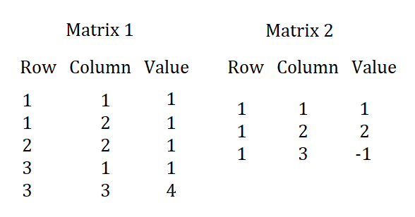
Consider the first matrix- matrix 1 in COO format

The second matrix- matrix-2 in COO format

We find the transpose of the second matrix - matrix2

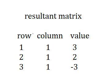
Now the resultant matrix in the COO format

resultant[1][1] = matrix1[1][1] * matrix2[1][1] + matrix[1][2] * matrix2[1][2] = 1 * 1 + 1 * 2 = 3

resultant[2][1] = matrix1[2][2] * matrix2[1][2] = 1 * 2 = 2

resultant[3][1] = matrix1[3][1] * matrix2[1][1] + matrix1[3][3] * matrix2[1][3] = 1 * 1 + 4 * -1 = 1 + (-4) = -3

resultant matrix is

Time complexity
Consider matrix A (m * n) and matrix B (n * k), with matrix A having a non-zero elements per column and matrix B with b non-zero elements per column. Then the total number of operations in multiplication of matrix A and matrix B is 2* n * a * b

Implementation
Implementation in Python using the Numpy library and the SciPy 2-D sparse array package for numeric data.
To peform sparse matrix multiplication, convert the matrix to CSR or CSC format using csr_matrix() function. It's used to create a sparse matrix of compressed sparse row format.

import numpy as np
from scipy.sparse import csr_matrix


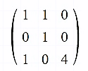
A = csr_matrix([[1, 1, 0], [0, 1, 0], [1, 0, 4]])
B = csr_matrix([[1, 0, 0], [2, 0, 0], [-1, 0, 0]])

print(np.dot(A.toarray(), B.toarray()))

Output:
[[ 3 0 0]
[ 2 0 0]
[-3 0 0]]

Sparse-Sparse matrix multiplication (SpGEMM)

• Sparse-Sparse matrix multiplications has many applications like graph processing, scientific computing, data analytics and so on.
• In the following research paper proposes a sparse-sparse matrix multiplication accelerator to improve performance. Here instead of using the inner and outer product which are inefficient to compute matrix multiplication, row-wise product is used leading to higher performance.
  https://ieeexplore.ieee.org/document/9251978

Sparse-Dense matrix multiplication (SpDM)

• Multiplication of a sparse matrix and a dense matrix has applications in scientific computing, machine learning and so on.
• A matrix is called a dense matrix if most of the elements are non-zero.
• The following research paper proposes an efficient sparse matrix-dense matrix multiplication algorithm on GPUs, called GCOOSpDM.
• Techniques used in the algorithm: coalesced global memory access, proper usage of the shared memory, and reuse the data from the slow global memory.
  https://ieeexplore.ieee.org/document/9359142

Dense-Sparse matrix product (DSMP)

• Here the first is dense and the second is sparse. It's needed to compute a sparse matrix chain product.
• The following research paper studies different versions of algorithms for optimizing dense-sparse matrix product for different compressed formats like CSR, DNS and COO.
  https://ieeexplore.ieee.org/document/8308259