
Get this book -> Problems on Array: For Interviews and Competitive Programming
In this article, we have explained the different cases like worst case, best case and average case Time Complexity (with Mathematical Analysis) and Space Complexity for Quick Sort. We will compare the results with other sorting algorithms at the end.
Table of Content:
- Basics of Quick Sort
- Time Complexity Analysis of Quick Sort
- Best case Time Complexity of Quick Sort
- Worst Case Time Complexity of Quick Sort
- Average Case Time Complexity of Quick Sort
- Space Complexity
- Comparison with other sorting algorithms
Basics of Quick Sort
Quick Sort is a sorting algorithm which uses divide and conquer technique.
In quick sort we choose an element as a pivot and we create a partition of array around that pivot. by repeating this technique for each partition we get our array sorted
depending on the position of the pivot we can apply quick sort in different ways
- taking first or last element as pivot
- taking median element as pivot
Pseduo Code:
quick_sort(array, start, end)
{
  if(start<end)
  {
    pivot_index = partition(array, start, end);
    quick_sort(array, start, pivot_index-1);
    quick_sort(array, pivot_index+1, end);
  }
}
Code:
#include<bits/stdc++.h>
using namespace std;
template<class T> void swap(T *a, T *b)
{
    T t = *a;
    *a = *b;
    *b = t;
}

int partition(int a[], int start, int end)
{
    int pivot = a[end];
    int i = (start-1);
    for(int j=start; j<=end-1; j++)
    {
        if(a[j]<=pivot)
        {
            i++;
            swap(&a[i], &a[j]);
        }
    }
    swap(a[i+1], a[end]);
    return (i+1);
}
void quick_sort(int a[], int start, int end)
{
    if(start<end)
    {
        int pivot_index = partition(a, start, end);
        quick_sort(a, start, pivot_index-1);
        quick_sort(a, pivot_index+1, end);
    }
}
int main()
{
  int a[] = {5, 2, 3, 4, 1, 6};
  int n = sizeof(a)/sizeof(a[0]);
  cout<<"Before"<<endl;
  for(int i=0; i<n; i++) cout<<a[i]<<" "; cout<<endl;
  quick_sort(a, 0, n-1);
  cout<<"After"<<endl;
  for(int i=0; i<n; i++) cout<<a[i]<<" "; cout<<endl;
  return 0;
}
Output:
Before
5 2 3 4 1 6
After
1 2 3 4 5 6
Time Complexity Analysis of Quick Sort
The average time complexity of quick sort is O(N log(N)).
The derivation is based on the following notation:
T(N) = Time Complexity of Quick Sort for input of size N.
At each step, the input of size N is broken into two parts say J and N-J.
T(N) = T(J) + T(N-J) + M(N)
The intuition is:
Time Complexity for N elements =
        Time Complexity for J elements +
        Time Complexity for N-J elements +
        Time Complexity for finding the pivot
where
- T(N) = Time Complexity of Quick Sort for input of size N.
- T(J) = Time Complexity of Quick Sort for input of size J.
- T(N-J) = Time Complexity of Quick Sort for input of size N-J.
- M(N) = Time Complexity of finding the pivot element for N elements.
Quick Sort performs differently based on:
- How we choose the pivot? M(N) time
- How we divide the N elements -> J and N-J where J is from 0 to N-1
On solving for T(N), we will find the time complexity of Quick Sort.
Best case Time Complexity of Quick Sort
-
O(Nlog(N))
-
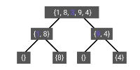
the best case of quick sort is when we will select pivot as a mean element.
-
In this case the recursion will look as shown in diagram, as we can see in diagram the height of tree is logN and in each level we will be traversing to all the elements with total operations will be logN * N
-
as we have selected mean element as pivot then the array will be divided in branches of equal size so that the height of the tree will be mininum
-
pivot for each recurssion is represented using blue color
-
time complexity will be O(NlogN)
Explanation
Lets T(n) be the time complexity for best cases
n = total number of elements
then
T(n) = 2*T(n/2) + constant*n
2*T(n/2) is because we are dividing array into two array of equal size
constant*n is because we will be traversing elements of array in each level of tree

therefore,
T(n) = 2*T(n/2) + constant*n
further we will devide arrai in to array of equalsize so
T(n) = 2*(2*T(n/4) + constant*n/2) + constant*n == 4*T(n/4) + 2*constant*n

for this we can say that
T(n) = 2^k * T(n/(2^k)) + k*constant*n
then n = 2^k
k = log2(n)

therefore,
T(n) = n * T(1) + n*logn = O(n*log2(n))
Worst Case Time Complexity of Quick Sort
-
O(N^2)
-
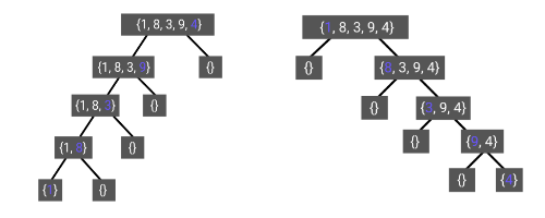
This will happen when we will when our array will be sorted and we select smallest or largest indexed element as pivot
as we can see in diagram we are always selecting pivot as corner index elements
so height of the tree will be n and in top node we will be doing N operations
then n-1 and so on till 1
Explanation
lets T(n) ne total time complexity for worst case
n = total number of elements

T(n) = T(n-1) + constant*n
as we are dividing array into two parts one consist of single element and other of n-1
and we will traverse individual array

T(n) = T(n-2) + constant*(n-1) + constant*n =  T(n-2) + 2*constant*n - constant
T(n) = T(n-3) + 3*constant*n - 2*constant - constant
T(n) = T(n-k) + k*constant*n - (k-1)*constant ..... - 2*constant - constant

T(n) = T(n-k) + k*constant*n - constant*[(k-1) ....  + 3 + 2 + 1]
T(n) = T(n-k) + k*n*constant - constant*[k*(k-1)/2]
put n=k
T(n) = T(0) + constant*n*n - constant*[n*(n-1)/2]
removing constant terms
T(n) = n*n - n*(n-1)/2
T(n) = O(n^2)
- we can reduce complexity for worst case by randomly picking pivot instead of selecting start or end elements
Average Case Time Complexity of Quick Sort
-
O(Nlog(N))
-
the overall average case for the quick sort is this which we will get by taking average of all complexities
Explanation
lets T(n) be total time taken

then for average we will consider random element as pivot
lets index i be pivot

then time complexity will be
T(n) = T(i) + T(n-i)

T(n) =  1/n *[\sum_{i=1}^{n-1} T(i)] + 1/n*[\sum_{i=1}^{n-1} T(n-i)]


As [\sum_{i=1}^{n-1} T(i)] and [\sum_{i=1}^{n-1} T(n-i)] equal likely functions
therefore
T(n) = 2/n*[\sum_{i=1}^{n-1} T(i)]

multiply both side by n
n*T(n) = 2*[\sum_{i=1}^{n-1} T(i)]      ............(1)

put n = n-1
  (n-1)*T(n-1) = 2*[\sum_{i=1}^{n-2} T(i)]      ............(2)

substract 1 and 2
then we will get
  n*T(n) - (n-1)*T(n-1) = 2*T(n-1) + c*n^2 + c*(n-1)^2
  n*T(n) = T(n-1)[2+n-1] + 2*c*n - c
  n*T(n) = T(n-1)*(n+1) + 2*c*n [removed c as it was constant]

divide both side by n*(n+1),
  T(n)/(n+1) = T(n-1)/n + 2*c/(n+1) .............(3)

put n = n-1,
  T(n-1)/n = T(n-2)/(n-1) + 2*c/n   ............(4)

put n = n-2,
  T(n-2)/n = T(n-3)/(n-2) + 2*c/(n-1)   ............(5)

by putting 4 in 3 and then 3 in 2 we will get
  T(n)/(n+1) = T(n-2)/(n-1) + 2*c/(n-1) + 2*c/n + 2*c/(n+1)

also we can find equation for T(n-2) by putting n = n-2 in (3)

at last we will get

  T(n)/(n+1) = T(1)/2 + 2*c * [1/(n-1) + 1/n + 1/(n+1) + .....]

  T(n)/(n+1) = T(1)/2 + 2*c*log(n) + C

  T(n) = 2*c*log(n) * (n+1)

now by removing constants,

  T(n) = log(n)*(n+1)

therefore,

  T(n) = O(n*log(n))
Space Complexity
-
O(N)
-
as we are not creating any container other then given array therefore Space complexity will be in order of N
Comparison with other sorting algorithms
| Algorithm | Average Time complexity | Best Time complexity | Worst Time complexity | Space complexity |
|---|---|---|---|---|
| Bubble sort | O(n^2) | O(n^2) | O(n^2) | O(n) |
| Heap Sort | O(n*log(n)) | O(n*log(n)) | O(n*log(n)) | O(n) |
| Merge Sort | O(n*log(n)) | O(n*log(n)) | O(n*log(n)) | Depends |
| Quicksort | O(n*log(n)) | O(n*log(n)) | O(n^2) | O(n) |
| Bubble sort | O(n^2) | O(n^2) | O(n^2) | O(n) |
With this article at OpenGenus, you must have the complete idea of Time and Space complexity analysis of Quick Sort.