In this article, we have explored Time and Space Complexity of Kruskal’s algorithm for MST (Minimum Spanning Tree). We have presented the Time Complexity of different implementations of Union Find and presented Time Complexity Analysis of Kruskal’s algorithm using it.

Table of contents:

1. Overview of Kruskal's algorithm
2. Time Complexity Analysis of Kruskal's Algorithm
3. Time complexity of Union function
4. Worst Case Time Complexity of Kruskal's Algorithm
5. Best Case Time Complexity of Kruskal's Algorithm
6. Average Case Time Complexity of Kruskal's Algorithm
7. Space Complexity of Kruskal's Algorithm
8. Conclusion

Prerequisite: Kruskal’s algorithm, Union Find, Minimum Spanning Tree

Overview of Kruskal's algorithm

Kruskal's algorithm is mainly used for finding a minimum spanning tree from a given graph. The given graph for finding MST is assumed to be connected and undirected.

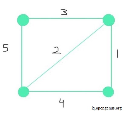
As shown in the above graph, the graph from which we create the MST is connected. It means that a path exists from each vertex to another vertex or vertices. Another feature of the given graph is that it's undirected. Meaning, the order in which the vertices connect is unimportant. The direction of the path is trivial, but a path must exist. For each path, we assign weights, as depicted along the paths in the graph above. We can refer to these paths as edges. From this graph, we create the MST.

All trees are data structures that contain no cycles. It implies that if we start following the path of any vertex and subsequent vertices after the said path, we won't end up at the same starting vertex. It means that no loops exist in a tree structure.

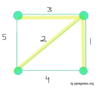
A spanning tree is a subgraph created from the main graph. Moreover, a spanning tree contains all vertices as in the main graph. A minimum spanning tree is also a subgraph of the main given graph. All vertices in the MST are connected. However, most importantly, an MST minimizes the sum of the weight of all edges taken together. The image below depicts an MST. The sum of all weights of each edge in the final MST is 6 (as a result of 3+2+1). This sum is the most minimum value possible.

Let the number of vertices in the given graph be V and the number of edges be E. In Kruskal's algorithm for MST, we first focus on sorting the edges of the given graph in ascending order. Then we start making the tree, adding the edge with the least weight first, and such that we form no cycles in the tree. We repeat this step till the number of edges in the MST becomes one less than the number of vertices V. That is, E becomes equal to V-1. Therefore, Kruskal's algorithm consists of the following main parts-

• Sort the edges in the given graph in an ascending order.
• Start making a spanning tree by adding the edge with the least weight first and check to make sure no cycles are formed.
• Repeat the previous step till the number of edges in the spanning tree is one less than the number of vertices in the main graph.

The pseudocode to implement this algorithm is explained below-

# an empty set for keeping final MST
S = {}

if edges not sorted: 
    Sort edges of the given graph per ascending order 

for every vertex (v) in given graph:
     create subset(v)

while number of edges < V-1:
    select edge having least weight
    if adding this edge doesn't create cycle:
        add edge to S
    increment the index to go to subsequent edge

# return final MST created
return S

This section briefly explained the fundamental ideas behind Kruskal's algorithm.

Time Complexity Analysis of Kruskal's Algorithm

In practice, while implementing Kruskal's algorithm, we keep track of all the edges using subsets. Using multiple subsets helps us to avoid cycles in our final MST output.

For this purpose, we make use of a data structure called Disjoint Sets or union-find. We store each edge as a set containing the two vertices and each of these sets contains elements. The disjoint set data structure then keeps a track of all these sets. This helps us to keep track of every set and makes sure every set is unique. To keep every set unique and make sure they don't contain the same elements, we merge unique elements into a single set.

For this purpose, we create a separate union function in Kruskal's algorithm. If we find overlapping elements in these sets, we don't include them in our disjoint set structure and don't call the union function, as it implies we have found a cycle.

In addition, we also create a find function, that helps us to find a particular's vertex set in the disjoint set structure. Using this function, if we find that two vertices are in the same set, we avoid using the union function and don't merge the two sets. This way we also make sure that all sets in the disjoint set data structure don't contain overlapping elements in them. Thus, using the disjoint set as our data structure, we can avoid cycles in our final MST.

Before making union and find functions, we also create a make_subset function, which creates a subset for each vertex of the edge. This helps us to later keep track of all edges and the sets created for our disjoint set structure.

To implement Kruskal's algorithm, we mainly focus on two functions to create our disjoint set structure-

• The make_subset function
• The find function
• The union function

It's important to note that before using these functions, we must first sort the edges as per the weights in ascending order. For that, we can use a simple algorithm like Merge sort, which has a time complexity of O(n(log(n)), where n stands for the number of nodes. So in this case, the runtime would be O(E(log(E)), where E is the number of edges.

Time complexity of make_set function
The make_set function is a fairly simple function that creates a subset for every vertex on the edge of the graph. The runtime for this function is constant O(1), since we take one vertex and turn it into a subset. Since we do it for all vertices, the total runtime becomes O(V).

Time complexity of Find function
The find function helps us to create a tree structure, keeps track of how each vertex in the edge is connected, gives us the subset that contains the vertex. We call this function for both vertices of each edge and check to see if they are in the same set in the disjoint set structure. If so, we ignore the edge and don't merge both sets into a single set. If not, then we merge them using the union function. This makes sure there are no overlapping elements in any set included in the disjoint set structure.

The find function creates a tree structure and we traverse the entire structure each time we call the function. So the complexity of this function for onetime is O(E or V), where E and V are the number of edges and vertices in the graph respectively.

We call this function for every vertex of each edge, the runtime of this function turns out to be O (E^2 or V^2), since the number of edges E are one less than the number of vertices V.

Time complexity of Union function

The union function takes the two vertices and in case they don't share the same set, we merge them into a single set. We call the union function for each edge that doesn't form a cycle. This function at most has a runtime of O(E) because to check the sets, we call the previous find function, and since we call this for all valid edges (edges that don't form cycle when adding to MST), the total runtime turns out to be O(E^2).

So in the end, the total time complexity, while also including the runtime for creating sets, sorting, along with the find and union function, becomes O(E(log(E) + E^2 + V)). Including only the high ordered terms, the runtime becomes O(E(log(E) + E^2)).

This is, however, a rudimentary implementation. We can make the performance much faster.

For better performance, we make use of a special form of a union called Union by Rank and for improving our find function, we implement Path Compression.

Path Compression
With this improvement, we link the lower level subtrees directly with the root parent node. For example, if 1 is connected with 2 and 2 is connected to 3, we directly connect 1 with 3. This way, we keep the height of the final tree as small as possible and 'compress' the path. Hence we call it path compression.

Improved Time Complexity of Find function
This improvement helps us to decrease the amount of time we spend traversing the tree to find the root of a vertex and subset of the disjoint set structure it's in. This way, we transform the height of the final tree into much less than that of a min-heap. Since we directly connect the lower nodes with the root, the height of the tree grows at a slow pace than log(V). Therefore, the runtime of the function turns out to be a constant in practice, O(1), much less than O(log(V)). In theory, we still assume it to be O(log(V)). Since we use this function for all vertices, total complexity turns out to be O(V(log(V)) or O(E(log(E)), since E is equal to V-1.

Union by Rank
When two sets don't contain overlapping elements and each element is part of a unique set, we merge the two sets into a single set in our disjoint set structure. When implementing union by rank, this time we keep track of each vertex's subtrees and keep track of their height.

Later on, when we merge the two sets, we merge them such that the tree with greater height becomes the parent of the tree with the smaller height. This way we cut the height of the overall tree structure that we create and it makes traversing and finding each vertex's set and parent node much easier.

This way, unlike the previous version of the union function, the height of the tree doesn't increase as much as it did before like a linked list.

Improved Time Complexity of Union function

As a result of a union by rank implementation of the union function, when we now check to see whether two vertices share the same set, we don't have to traverse a big linked list-like tree. Since now we directly attach the subtree with small height as the child of the tree with greater height when merging, the resulting structure height becomes much like a heap, and even better.

We cut the height of the tree by more than half each time and therefore, the runtime, although sometimes assumed as O(log(n)), is much less than that. The final tree structure we use to keep track of all vertices and their parents grows at a very small pace.

Therefore, in many practical executions, we assume the final runtime of this union function as O(1) or constant. But in theory, we assume it as O(log(n)). When we call this function V-1 times for all edges E, the total runtime becomes-

• O(log(E)) at maximum for first iteration
• O(log(E)) at maximum for second iteration
• and so on for V-1 number of times, which is E

So mathematically, the total final complexity for this function turns out to be O(E(log(E)).

Therefore, taking into account sorting, make_set function's runtime and then the improved union and find function, that total runtime turns out to be O(E(log(E) + V + E(log(E)) + E(log(E))) leading to final complexity of O(E(log(E)).

Worst Case Time Complexity of Kruskal's Algorithm

The worst case might happen when all the edges are not sorted, the graph contains maximum number of edges, and we have included the edge with maximum weight in our MST. So in this case, we would need to check all the edges at each step to make sure our MST includes minimal weighted edges. The maximum possible number of edges in an undirected graph is given by n(n-1)/2. Ignoring constants, this results in n^2 total maximum number of edges. Such a graph having maximum number of edges is called a Dense graph. In such a case, the graph with V number of vertices would have V^2 number of edges.

This is the worst case because the two most important parts in this algorithm are - sorting the edges and checking if each edge forms no cycle to then add to MST, so performance is mostly dependent on the number of edges and weights. Hence a dense graph would have a significant impact on runtime. The image below depicts an example of a dense graph.

In such a case, for all vertices V and edges E-

• Sorting edges using merge sort would take O(E(log(E)) time
• The function make_set would take at max runtime of O(V), as it creates a subset for all vertices
• The improved functions union and find will make sure the final tree structure stays at a minimal height, therefore at max, the runtime of both functions becomes O(E(log(E)) overall.

Therefore, in the worst case, the total complexity turns out to be O(E(log(E)).

Best Case Time Complexity of Kruskal's Algorithm

In the best case, we assume the edges E are already sorted and we have a graph having minimum number of edges as possible. A graph with minimal number of edges is called a Sparse graph. An example of such a graph is shown below.

In such a case, we won't need to sort edges and the impact of edges on the rest of the algorithm will be minimal in practice but same as worst case in theory.

Another case could be when the first V-1 edges form the MST. That way, the number of operations for all edges would be minimum.

In either of the above two cases-

• The make_set function would have a runtime same as the worst case, O(V).
• The union and find functions would have a constant runtime in practice but Log(E) runtime in theory. Considering that we do this for all vertices and valid edges, the total complexity for each would be O(E(log(E)).

Therefore, the total time complexity in the best case becomes O(E(log(E)), since E is V-1.

Average Case Time Complexity of Kruskal's Algorithm

Considering all forms of graphs we might come across as input for this algorithm-

• The sorting and make_set function would have the same runtime on average as the worst, if we don't consider the constants.
• In functions union and find, we either consider two vertices (parent and the current node) or two subtrees at a time. So the complexity would be a constant in practice, but (log E) in theory, divided by two on average per operation. Ignoring the constants, the runtime would be the same as the worst case.

Therefore, the total runtime on average would also be O(E(log(E)).

Space Complexity of Kruskal's Algorithm

The special structure that we use to keep track of all vertices, edges in a tree form called the Disjoint set structure, requires-

• A space requirement of O(V) to keep track of all vertices in the beginning and the respective subsets.
• A space requirement of O(E) to keep track of all the valid sorted edges to be included in the final MST.

Therefore, the total space complexity turns out to be O(E+V).

Conclusion

In summary, Kruskal's algorithm requires-

• A worst-case time complexity of O(E(log(E)).
• An average-case time complexity of O(E(log(E)).
• A best-case time complexity of O(E(log(E)).
• A space complexity of O(E+V).

With this article at OpenGenus, you must have the complete idea of Time and Space Complexity of Kruskal’s algorithm for MST.