Open-Source Internship opportunity by OpenGenus for programmers. Apply now.
Reading time: 35 minutes
We have explored implementing Linear Regression using TensorFlow which you can check here, so first we will walk you though the difference between Linear and Logistic Regression and then, take a deep look into implementing Logistic Regression in Python using TensorFlow.
Read about implementing Linear Regression in Python using TensorFlowIn the first article, we used a random dataset with 100 datapoints between 0 and 25, and the Linear Regression could find the Regression Line, considering the mean of all the values.
If we consider that dataset as a Train Set, we could predict more values in a Test or Real environment, and it would be all between 0 and 25, including decimal numbers like 0.25, 3.20, 19.99 just to give some examples.
When we go to Logistic Regression, we are talking about a Classification algorithm, which will give us a result like 0 or 1, which can mean Yes or No, Higher or Lower, Approved or Not Approved, etc. The main objective is draw a decision boundary in our dataset. Everything from one side receive one classification, everything from the other side receives other classification. Lets see how we can do this using Python and TensorFlow library.
import numpy as np
import pandas as pd
import tensorflow as tf
import matplotlib.pyplot as plt
First thing, imports all libraries that we will need. Numpy for create the arrays, TensorFlow to do the regression, Matplotlib to plot data, Pandas to interact with the Dataframe.
df = pd.read_csv('../Iris.csv')
Creating our Dataframe using the Iris dataset.
Above you have to put the correct path of your CSV file, that you can download here
This dataset have 3 Species of Iris Flower. The first one, Setosa is linearly separable from Versicolor and Virginica. But the last 2 are not linearly separable from eachother. Considering we have 50 samples of each, and the dataset is ordered, lets slice the dataset and consider only the first 100 rows, it will give us 2 Species linearly separale. In the real world, with more complex datasets, you may have a lot of more work to do it, but Pandas can be the life saver in those situations.
df = df[:100]
df.shape
Output:
Now in order to do our regression, we need replace the Species in 0 and 1
df.Species = df.Species.replace(to_replace=['Iris-setosa', 'Iris-versicolor'], value=[0, 1])
Above I have changed Iris-setosa to 0, and Iris-versicolor to 1
df.head()
Output:
plt.scatter(df[:50].SepalLengthCm, df[:50].SepalWidthCm, label='Iris-setosa')
plt.scatter(df[51:].SepalLengthCm, df[51:].SepalWidthCm, label='Iris-versicolo')
plt.xlabel('SepalLength')
plt.ylabel('SepalWidth')
plt.legend(loc='best')
Plot of our data. It is easy to see that we have 2 different classes.
Output:
X = df.drop(labels=['Id', 'Species'], axis=1).values
y = df.Species.values
Creating our variables: Features
Xand our targety.
seed = 23
np.random.seed(seed)
tf.set_random_seed(seed)
Setting a seed to reproducibility (use the same seed as me to have same results).
train_set = np.random.choice(len(X), round(len(X) * 0.4), replace=False)
Creating the train set considering 40% of the data.
test_set = np.array(list(set(range(len(X))) - set(train_set)))
train_X = X[train_set]
train_y = y[train_set]
test_X = X[test_set]
test_y = y[test_set]
Creating the test set considering 60% of the data, and train and test variables.
def min_max_normalized(data):
    col_max = np.max(data, axis=0)
    col_min = np.min(data, axis=0)
    return np.divide(data - col_min, col_max - col_min)
Define the normalized function.
train_X = min_max_normalized(train_X)
test_X = min_max_normalized(test_X)
Normalized processing, must be placed after the data set segmentation,
otherwise the test set will be affected by the training set.
A = tf.Variable(tf.random_normal(shape=[4, 1]))
b = tf.Variable(tf.random_normal(shape=[1, 1]))
init = tf.global_variables_initializer()
sess = tf.Session()
sess.run(init)
Declare the variables that need to be learned and initialization
data = tf.placeholder(dtype=tf.float32, shape=[None, 4])
target = tf.placeholder(dtype=tf.float32, shape=[None, 1])
Define placeholders
Placeholders?
A placeholder works like any other variable, but it doesn´t need a initial value.
mod = tf.matmul(data, A) + b
Declare the model you need to learn
loss = tf.reduce_mean(tf.nn.sigmoid_cross_entropy_with_logits(logits=mod, labels=target))
Declare the loss function
Loss Function?
This formula is used to determine the value of the weight and bias from the given dataset.
learning_rate = 0.003
batch_size = 30
epoch_iter = 1500
Defining parameters:
Learning Rate?
Learning rate is a hyper-parameter that controls how much we are adjusting the weights of our network with respect the loss gradient.
Batch Size?
The batch size defines the number of samples that will be propagated through the network.
Epoch?
An epoch is a full iteration over samples.
opt = tf.train.GradientDescentOptimizer(learning_rate)
Defining the optimizer
Gradient Descent Optimizer?
It is an alghoritm that is used to find the optimized paramaters.
goal = opt.minimize(loss)
Defining Goal
prediction = tf.round(tf.sigmoid(mod))
correct = tf.cast(tf.equal(prediction, target), dtype=tf.float32)
accuracy = tf.reduce_mean(correct)
Defining accuracy
loss_trace = []
train_acc = []
test_acc = []
Creating variables to store the results
for epoch in range(epoch_iter):
    # Generate random batch index
    batch_index = np.random.choice(len(train_X), size=batch_size)
    batch_train_X = train_X[batch_index]
    batch_train_y = np.matrix(train_y[batch_index]).T
    sess.run(goal, feed_dict={data: batch_train_X, target: batch_train_y})
    temp_loss = sess.run(loss, feed_dict={data: batch_train_X, target: batch_train_y})
    # convert into a matrix, and the shape of the placeholder to correspond
    temp_train_acc = sess.run(accuracy, feed_dict={data: train_X, target: np.matrix(train_y).T})
    temp_test_acc = sess.run(accuracy, feed_dict={data: test_X, target: np.matrix(test_y).T})
    # recode the result
    loss_trace.append(temp_loss)
    train_acc.append(temp_train_acc)
    test_acc.append(temp_test_acc)
    # output
    if (epoch + 1) % 300 == 0:
        print('epoch: {:4d} loss: {:5f} train_acc: {:5f} test_acc: {:5f}'.format(epoch + 1, temp_loss,
                                                                          temp_train_acc, temp_test_acc))
Training the model
Output:
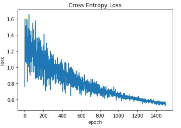
plt.plot(loss_trace)
plt.title('Cross Entropy Loss')
plt.xlabel('epoch')
plt.ylabel('loss')
plt.show()
Plot of the loss function
Output:
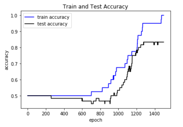
plt.plot(train_acc, 'b-', label='train accuracy')
plt.plot(test_acc, 'k-', label='test accuracy')
plt.xlabel('epoch')
plt.ylabel('accuracy')
plt.title('Train and Test Accuracy')
plt.legend(loc='best')
plt.show()
Plot of the accuracy
Output:


