In this article, we have explored the basics of Mathematics for Computational Geometry including Points, Lines, Angles, Circle, Triangle and other topics.

Table of Contents

• Introduction
• Points
• Lines and Curves
• Angles
• Vectors
• Circles
• Triangles
• Overview

Introduction

Geometry is a branch of mathematics which is concerned with the properties, angles, measurements, shape and size of space. Generally, geometry is fundamentally based on points, lines and planes in a given space. In most cases, we will be dealing with Euclidean geometry. This is the form of geometry that the vast majority of people are familiar with in their everyday lives. We can categorise geometry in two ways, plane and solid.

Plane geometry is focused around shapes on a two dimensional surface that extends infinitely. A two-dimensional shape is one that does not have existing depth, only length and height. This includes shapes such as a triangle, square or circle.

Solid geometry therefore, is concerned around shapes with three dimensions, length, height and width. We can include in this category shapes such as spheres, pyramids or cubes. These shapes have properties such as faces, corners and vertices all of which are analysed when we begin to solve solid geometry problems.

Points

As stated in the introduction, a shape can have length and height dimensions if it is 2D, with the added width dimension in 3D. These can be expressed as co-ordinate points x (length), y (height), z (width). A singular point contains an x, y and z value which then can be expressed in space, for 2D shapes, the z value is always 0.

Lines and Curves

In 2D geometry, when two points are connected to each other, this is called a line. A line will have an equation which represents how it is drawn, from this we can calculate the location of any point along said line or curve. For a straight line this equation can be defined broadly as:

y = mx + c 

Where:

• m is the gradient
• c is the point where y crosses the y axis (y-intercept)

We can also find the equation of a straight line if we have an x and y co-ordinate point by using this formula

y - y1 = m(x - x1)

Where x1 and y1 are the co-ordinates and m is the gradient

For a straight line, we can find the gradient (rate of change) of the line using a simple formula

m = delta(y)/delta(x) = (y2-y1)/(x2-x1)

For a curve we should use differentiation of the equation

m = dy/dx

We can find the midpoint of a line by using the formula:

(xm, ym) = ((x1 + x2)/2, (y1 + y2)/2)

Where x1,x2,y1,y2 are the respective points of the line

Finally, we can also find the distance between two points using this formula:

d = √((x2-x1)²+(y2-y1)²)

This formula is a rearrangement of the Pythagorean theorem.

Angles

Angles are the figures formed from two rays, or lines which originate from the same vertex. They can also be formed from two planes intersecting. They can be measured usually in degrees or radians.

Angles can give shapes certain properties, for example, the angles inside a triangle will always add to 180 degrees. Angles that are located within a shape are called interior and those around the outside are named exterior. We can generalise an equation in order to find how many degrees the sum of the interior and exterior angles of a shape with equal, if we know the number of sides

Interior: (n - 2) * 180 degrees
Exterior: 360 degrees for all polygons
Where n is number of sides

To find the size of individual angles we simply have to divide the number of sides by the sum of the angles.

Vectors

A vector is a structure that we use when solving geometry problems. A vector has both direction and magnitude, meaning that it can act as a certain force in a direction. When we write vectors, usually it is in component form, this represents the influence that the vector will have in a given direction.

An example of this for a 3D vector could be:

v = v_xi + v_yj v_zk

We can carry out operations on vectors too. Vector addition is used to determine the resultant force of multiple vectors and can be carried out simply like standard addition, giving us a new vector

v1 = (5,4)
v2 = (6,3)
v1 + v2 = v3 (5 + 6, 4 + 3)
v3 = (11, 7)

The same principles would apply for subtraction. We will cover more advanced vector operations later on.

2D shapes

In this section we will cover some introductory operations and formulas used with some 2D shapes.

Circle

A circle can be dissected into some main sections which include:

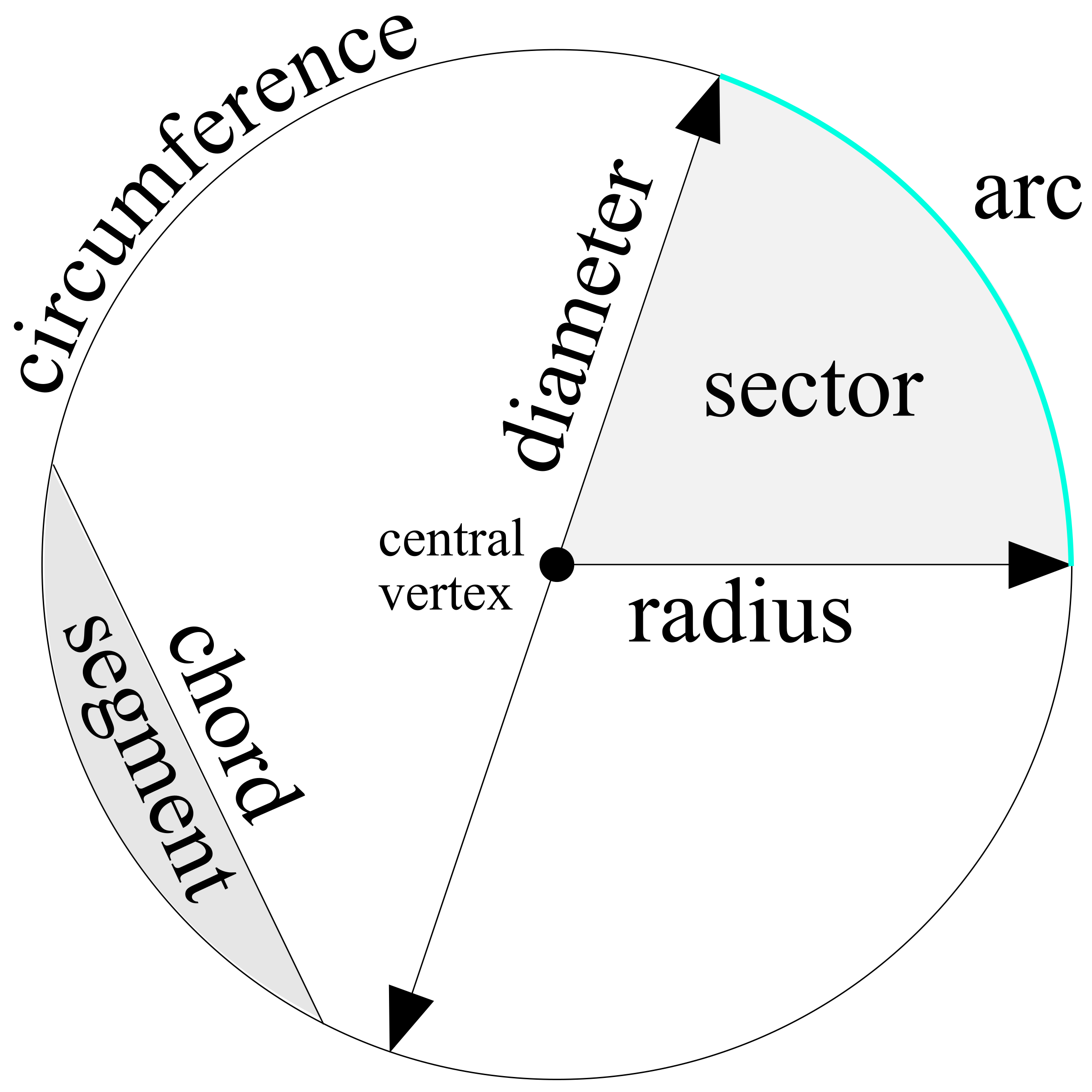
Each of these parts of a circle interact with each other and can be used in order to find its key properties.

The area of a circle can be calculated using the equation:

A = πr2
Where r is the radius

We use π in this formula as it is the ratio of the circumference to the diameter of any circle.

We can calculate the circumference using:

C = 2πr

These are the two most basic formulas in regards to circles, and will be used extensively in many areas.

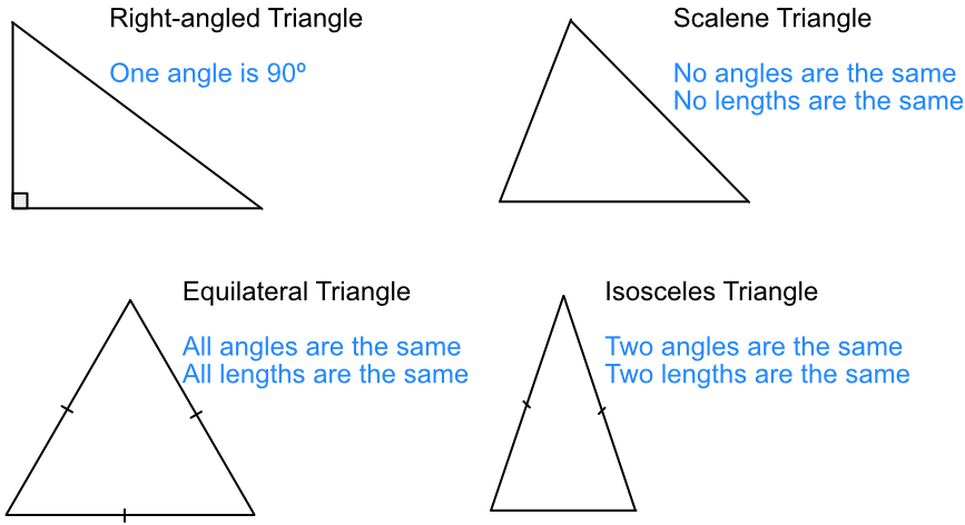
Triangle

There are multiple different types of triangle with various different properties:

The area of a triangle can be calculated by using the formula:

A = (Base * Height)/2

We use this formula since the diagonal of a rectangle forms two congruent triangles (meaning they are equivalent), and the area of a rectangle is W * H, so to find only one of these diagonals, we simply divide by 2.

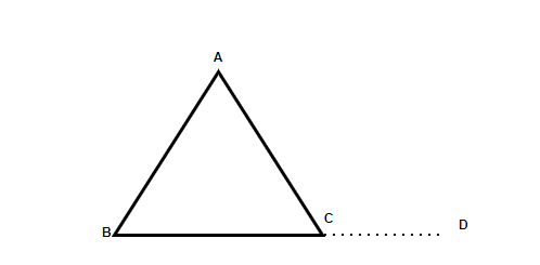
Here is another diagram of a triangle, we can use this to derive some properties:

• Interior angles add to 180 degrees, therefore the interior angles of a triangle are more than 0 degrees and less than 180 degrees
• The exterior angle of a triangle is equal to the sum of the opposite and non-adjacent angle in the interior eg. ∠ACD = ∠ABC + ∠BAC
• The side opposite to the largest angle will therefore be the longest side
• For triangles to be similar, their angles have to be congruent and the sides proportional to each other.

Overview

We have given a basic overview of geometry and a good foundation into further exploration of the topic. We have described fundamental principles such as points, lines, angles, vectors and more, whilst also giving useful equations which will become key in future work. Finally, we have covered some 2D shapes and the inherent properties that come with it, this will come in useful later to use when designing algorithms.