
In this article, we have explored how to compare two different audio in Python using librosa library.
Table of contents:
- Waveforms and domains
- Oboe
- Clarinet
- Time Stretch
- Log Power Spectrogram
- MFCC
Waveforms and domains
Waveform wrt sound represents movement of particles in a gaseous, liquid, or solid medium.
Time domain when refering wrt sound is depection of particles movement with the help of analysis of time.
Frequency domain when refering wrt sound is depection of particles movement with the help of analysis of frequency (explained later).
CODE
#Time Domain
import numpy as np
import matplotlib.pyplot as plt
from glob import glob
import librosa as lr
import librosa.display
from IPython.display import Audio
import IPython.display as ipd

audio1='First'
y, sr = lr.load('./{}.wav'.format(audio1))
ipd.Audio(y, rate=sr)
plt.figure(figsize=(15, 5))
lr.display.waveplot(y, sr, alpha=0.8)
plt.show()

audio2='Second'
y, sr = lr.load('./{}.wav'.format(audio2))
ipd.Audio(y, rate=sr)
plt.figure(figsize=(15, 5))
lr.display.waveplot(y, sr, alpha=0.8)
plt.show()
Output :
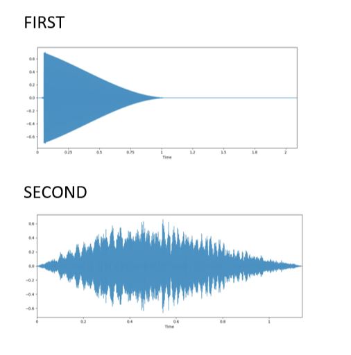
In the output of first audio we can predict that the movement of particles wrt time is gradually decreasing. Hence formation of a triangle. While for second audio the movement of particle first increases and then decreases.
Frequency Domain
import numpy as np
import matplotlib.pyplot as plot
from scipy import pi
from scipy.fftpack import fft
import librosa as lr
import librosa.display

audio1='First'
y, sr = lr.load('./{}.wav'.format(audio1))
signalAmplitude   = np.sin(y)
plot.subplot(211)
plot.plot(y, signalAmplitude,'bs')
plot.xlabel('time')
plot.ylabel('amplitude')
plot.subplot(212)
plot.magnitude_spectrum(signalAmplitude,Fs=4)
plot.show()

audio2='Second'
y, sr = lr.load('./{}.wav'.format(audio2))
signalAmplitude   = np.sin(y)
plot.subplot(211)
plot.plot(y, signalAmplitude,'bs')
plot.xlabel('time')
plot.ylabel('amplitude')
plot.subplot(212)
plot.magnitude_spectrum(signalAmplitude,Fs=4)
plot.show()
Output :
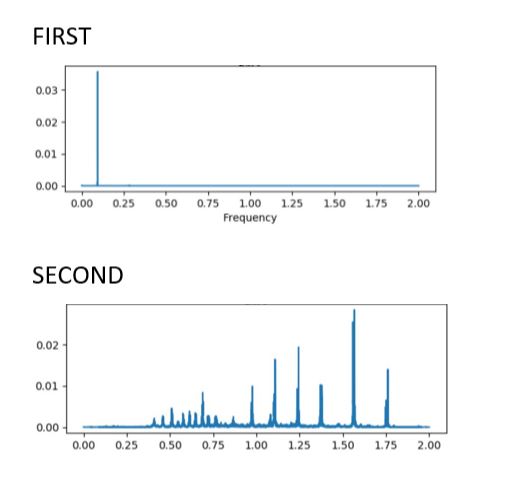
From the output we can say that First is having a constant movement of partiles except at one significant point while for Second we are having many back and forth movement of particles.
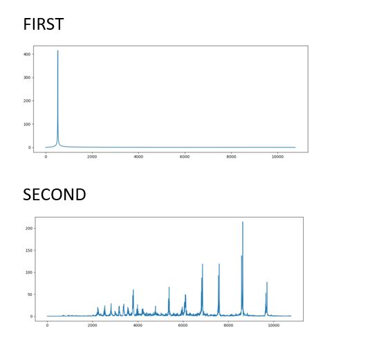
Oboe
Oboe is an instrument which is placed between the lips and blown which causes both reeds to vibrate against each other. They open and close very rapidly, sending bursts of energy into the air column inside the instrument and causing it to vibrate in sympathy.
We now potray the movement of particles of our audio when passed through oboe.
Code
import numpy as np
import matplotlib.pyplot as plt
from glob import glob
import librosa as lr
import librosa.display
from IPython.display import Audio
import IPython.display as ipd
import scipy

audio1='First'
y, sr = lr.load('./{}.wav'.format(audio1))
f = np.linspace(0, sr, 4096)
print(y.shape)
X = scipy.fft(y[10000:14096])
X_mag = np.absolute(X)
plt.figure(figsize=(14, 5))
plt.plot(f[:2000], X_mag[:2000]) # magnitude spectrum
plt.xlabel('Frequency (Hz)')
plt.show()

audio2='Second'
y, sr = lr.load('./{}.wav'.format(audio2))
f = np.linspace(0, sr, 4096)
print(y.shape)
X = scipy.fft(y[10000:14096])
X_mag = np.absolute(X)
plt.figure(figsize=(14, 5))
plt.plot(f[:2000], X_mag[:2000]) # magnitude spectrum
plt.xlabel('Frequency (Hz)')
plt.show()
Output :
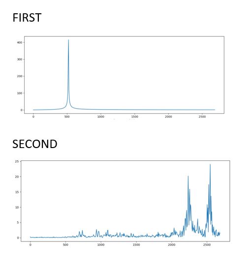
Clarinet
It is a single-reed woodwind instrument used orchestrally and in military and brass bands and possessing a distinguished solo repertory.
We now potray the movement of particles of our audio when passed through clarinet.
CODE
import numpy as np
import matplotlib.pyplot as plt
from glob import glob
import librosa as lr
import librosa.display
from IPython.display import Audio
import IPython.display as ipd
import scipy

audio1='First'
y, sr = lr.load('./{}.wav'.format(audio1))
f = np.linspace(0, sr, 4096)
ipd.Audio(y, rate=sr)
print(y.shape)
X = scipy.fft(y[10000:14096])
X_mag = np.absolute(X)
plt.figure(figsize=(14, 5))
plt.plot(f[:500], X_mag[:500]) # magnitude spectrum
plt.xlabel('Frequency (Hz)')
plt.show()

audio2='Second'
y, sr = lr.load('./{}.wav'.format(audio2))
f = np.linspace(0, sr, 4096)
ipd.Audio(y, rate=sr)
print(y.shape)
X = scipy.fft(y[10000:14096])
X_mag = np.absolute(X)
plt.figure(figsize=(14, 5))
plt.plot(f[:500], X_mag[:500]) # magnitude spectrum
plt.xlabel('Frequency (Hz)')
plt.show()
Output :
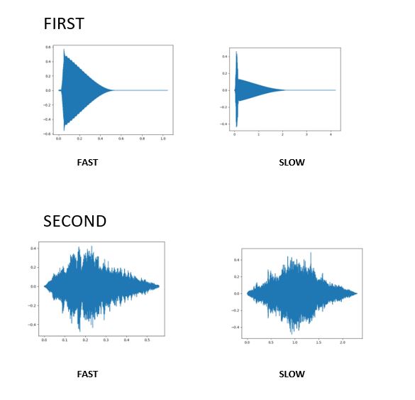
Time Stretch
In this code we have increased the time that is twice the speed of original audio and decreses the time as well by half.
CODE
import numpy as np
import matplotlib.pyplot as plt
from glob import glob
import librosa as lr

audio1='First'
y, sr = lr.load('./{}.wav'.format(audio1))
y_fast = lr.effects.time_stretch(y, 2.0)
time = np.arange(0,len(y_fast))/sr
fig, ax = plt.subplots()
ax.plot(time,y_fast)
ax.set(xlabel='Time(s)',ylabel='sound amplitude')
plt.show()

y_slow = lr.effects.time_stretch(y, 0.5)
time = np.arange(0,len(y_slow))/sr
fig, ax = plt.subplots()
ax.plot(time,y_slow)
ax.set(xlabel='Time(s)',ylabel='sound amplitude')
plt.show()

audio2='Second'
y, sr = lr.load('./{}.wav'.format(audio2))
y_fast = lr.effects.time_stretch(y, 2.0)
time = np.arange(0,len(y_fast))/sr
fig, ax = plt.subplots()
ax.plot(time,y_fast)
ax.set(xlabel='Time(s)',ylabel='sound amplitude')
plt.show()

y_slow = lr.effects.time_stretch(y, 0.5)
time = np.arange(0,len(y_slow))/sr
fig, ax = plt.subplots()
ax.plot(time,y_slow)
ax.set(xlabel='Time(s)',ylabel='sound amplitude')
plt.show()
Output :
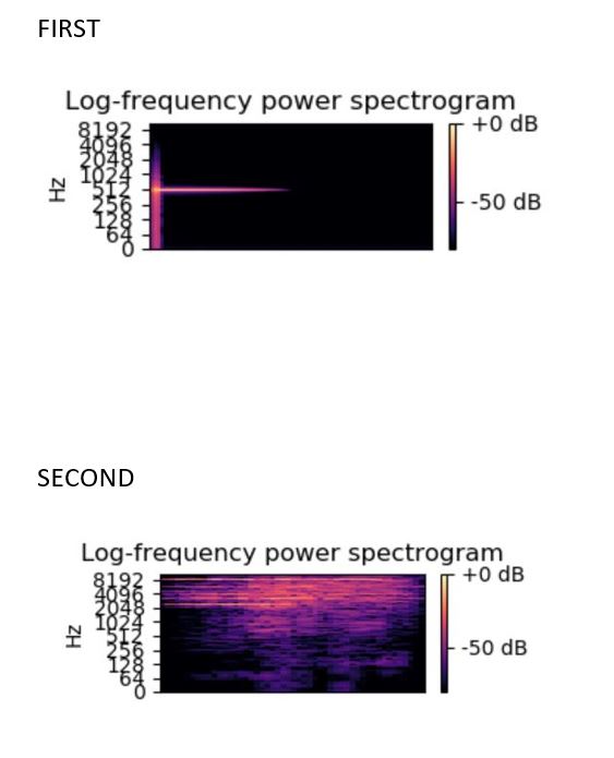
Log Power Spectrogram
The Log Power Spectrogram is used to demonstrate the distribution of power across frequency components of a given signal.
As we know, any audio signal can be split into multiple signals having different frequencies or a range of frequencies. This is proved using Fourier Analysis.
CODE
import numpy as np
import matplotlib.pyplot as plt
from glob import glob
import librosa as lr
import librosa.display
audio1='First'
y, sr = lr.load('./{}.wav'.format(audio1))
D = librosa.amplitude_to_db(np.abs(librosa.stft(y)), ref=np.max)
plt.subplot(4, 2, 2)
lr.display.specshow(D, y_axis='log')
plt.colorbar(format='%+2.0f dB')
plt.title('Log-frequency power spectrogram')
plt.show()

audio2='Second'
y, sr = lr.load('./{}.wav'.format(audio))
D = librosa.amplitude_to_db(np.abs(librosa.stft(y)), ref=np.max)
plt.subplot(4, 2, 2)
lr.display.specshow(D, y_axis='log')
plt.colorbar(format='%+2.0f dB')
plt.title('Log-frequency power spectrogram')
plt.show()
Output :
MFCC
The output of the below code is .txt file which is no included here but uploaded in our GitHub account do give it a look.
Code
import librosa
import numpy as np

RATE = 24000
N_MFCC = 13

def get_wav(language_num):
    '''
    Load wav file from disk and down-samples to RATE
    :param language_num (list): list of file names
    :return (numpy array): Down-sampled wav file
    '''

    y, sr = librosa.load('./{}.wav'.format(language_num))
    return(librosa.core.resample(y=y,orig_sr=sr,target_sr=RATE, scale=True))

def to_mfcc(wav):
    '''
    Converts wav file to Mel Frequency Ceptral Coefficients
    :param wav (numpy array): Wav form
    :return (2d numpy array: MFCC
    '''
    return(librosa.feature.mfcc(y=wav, sr=RATE, n_mfcc=N_MFCC))

if __name__ == '__main__':

    audio1 = 'First'
    X= get_wav(audio1)
    X=to_mfcc(X)
    c = np.savetxt('file1.txt', X, delimiter =', ')
    a = open("file1.txt", 'r')# open file in read mode

    audio2 = 'Second'
    X= get_wav(audio2)
    X=to_mfcc(X)
    c = np.savetxt('file2.txt', X, delimiter =', ')
    a = open("file2.txt", 'r')# open file in read mode


    print("the file contains:")
    print(a.read())
With this article at OpenGenus, you must have the complete idea of how to compare to audio in Python using librosa library.