In this article, we have explained the different cases like worst case, best case and average case Time Complexity (with Mathematical Analysis) and Space Complexity for Merge Sort. We will compare the results with other sorting algorithms at the end.

Table of Content:

1. What is Merge sort
2. Pseudo code of merge sort
3. Implementation of merge sort
4. Time Complexity Analysis of Merge Sort
5. Best case Time Complexity of Merge Sort
6. Worst Case Time Complexity of Merge Sort
7. Average Case Time Complexity of Merge Sort
8. Space Complexity
9. Comparison with other sorting algorithms

Prerequisite: Merge Sort

In short,

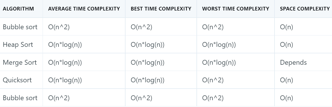
Case	Time Complexity	# Comparisons	When?
Worst Case	O(N logN)	N logN	Specific distribution
Average Case	O(N logN)	0.74 NlogN	Average
Best Case	O(N logN)	0.50 NlogN	Already sorted

• Space Complexity: O(N)

Let us get started with Time & Space Complexity of Merge Sort.

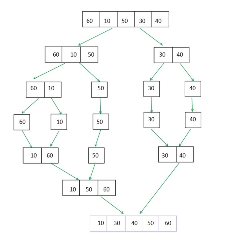
Overview of Merge Sort

In simple terms merge sort is an sorting algorithm in which it divides the input into equal parts until only two numbers are there for comparisons and then after comparing and odering each parts it merges them all together back to the input.

PSEUDO CODE OF MERGE SORT

  MergeSort(vector<int> input, left,  right)
  // intially left =0 and right = input.size()-1;
If right > left
     1. Find the middle point to divide the input into two halves:  
             middle = left+ (right-left)/2
     2. Call MergeSort for first half:   
             Call MergeSort(input, left, middle)
     3. Call MergeSort for the other half:
             Call MergeSort(input, middle+1, right)
     4. Merge the two halves sorted in step 2 and 3:
             Call Merge(input, left, middle, right)

IMPIMPLEMENTATION

#include<bits/stdc++.h>
#define ll long long int
using namespace std;
void merge(vector<int> &input, int left, int middle, int right)
{
    int n =middle-left+1; // size of first array
    int m =right -middle; //size of rest of the elements
    int first[n];
    for(int i=0;i<n;i++)
    {
    
        first[i]=input[left+i];
        //cout<<first[i]<<" ";
    }
   // cout<<endl;
   int rest[m];
     for(int i=0;i<m;i++)
    {
        rest[i]=input[middle+1+i];
        //cout<<rest[i]<<" ";
    }
   // cout<<endl;
    int ptr1=0;
    int ptr2=0;
    int index=left;
    // MERGE PROCESS WITH COMPARISONS 
    while(ptr1<n && ptr2<m)
    {
        if(first[ptr1] < rest[ptr2])
        {
            input[index]=first[ptr1];
            index++;
            ptr1++;
        }
        else 
        {
             input[index]=rest[ptr2];
            index++;
            ptr2++;
        }
    }
    while(ptr1 < n)
    {
        input[index]=first[ptr1];
            index++;
            ptr1++;
    }
    while(ptr2 < m)
    {
        input[index]=rest[ptr2];
            index++;
            ptr2++;
    }
}
void solve(vector<int>&input, int left, int right)
{
   if(left < right)
   {
      // LETS DIVIDE
      int middle =(left+right)/2;
      solve(input,left,middle);
      solve(input,middle+1,right);
      // after dividing lets merge it
      merge(input,left,middle,right);        
   }
}
int main()
{
    int n;
    cin>>n;
    vector<int> input;
    for(int i=0;i<n;i++)
    {
        int x;
        cin>>x;
        input.push_back(x);
    }
    solve(input,0,n-1);
    // AFTER SORTING
     for(int i=0;i<n;i++)
    {
        cout<<input[i]<<" ";
    }
    cout<<endl;
    
   
    return 0;
}

OUTPUT

5
1 5 2 7 8
AFTER SORTING
1 2 5 7 8 

Time Complexity Analysis of Merge Sort

Now, let us follow up with the steps. our very own first step was to divide the input into two halves which comprised us of a logarithmic time complexity ie. log(N) where N is the number of elements.

our second step was to merge back the array into a single array, so if we observe it in all the number of elements to be merged N, and to merge back we use a simple loop which runs over all the N elements giving a time complexity of O(N).
finally, total time complexity will be - step -1 + step-2

General analysis

T(N) = Time Complexity for problem size N
T(n) = Θ(1) + 2T(n/2) + Θ(n) + Θ(1)
T(n) = 2T(n/2) + Θ(n)

Let us analyze this step by step:
T(n) = 2 * T(n/2) + 0(n)

STEP-1 Is to divide the array into two parts of equal size .
2 * T(n/2) --> Part 1

STEP-2 Now to merge baiscall traverse through all the elements.
constant * n --> Part 2

STEP-3 --> COMBINE 1 + 2
T(n) = 2 * T(n/2) + constant * n --> Part 3

Now we can further divide the array into two halfs if size of the partition arrays are greater than 1. So,

n/2/2--> n/4
T(N) = 2 * (2 * T(n/4) + constant * n/2) + constant * n
T(N) = 4 * T(n/4) + 2 * constant * n

For this we can say that:
Where n can be subtituted to 2^k and the value of k is logN
T(n) = 2^k * T(n/(2^k)) + k * constant * n

Hence,
T(N) = N * T(1) + N * logN
= O(N * log(N))

LETS TALK IN MORE DETAIL ABOUT IT

Best Case Time Complexity of Merge Sort

For the best case, one can assume that the array is already sorted so in that case the number of comparisons would be minimum.

In Merge Sort, the comparisons take place in the merge step. If there are two sorted arrays of size M, the minimum number of comparisons will be M. This will happen when all elements of the first array is less than the elements of the second array.

So, the first element of the 2^nd array is compared with each element of the first array and then, the 2^nd array is attached at the end of 1^st array.

At every step, only N/2 elements are compared and there are O(logN) such steps.

Let uss take an example

INPUT - [1,2,3,4,5]
STEP -1 divide it into equal parts
[1,2,3] and [4,5]

We can see that it can be further divided into smaller parts
[1,2] [3] [4,5]
Intially, let us assume that the count of swaps is 0, now if we check for the condition where first < second and if not than we increase the count swap by 1.
[1,2] == first < second count=0;
[3] == only one element so no comparisons count=0;
[4,5] == first < second count=0;
// Now we have
[1,2] [3] [4,5]
Now lets merge back all the parts into one sorted array
[1,2,3,4,5]--> one can see that there is no swaps required in merging as well.

Therefore in Best Case,

• Input is already sorted
• Best Case Time Complexity: O(N logN)
• Number of Comparisons: 0.5 N logN

Average Case Time Complexity of Merge Sort

Number of comparisons decide the complexity to be best , average or worst.

INPUT - [1,3,4,11,7,9,5]
// we can clearly see that one part is going to have more elements so if we split it into two possible way

OPTION-1
[1,3,4] and [11,7,9,5]
we can see that it can be further divided into smaller parts
[1,3] [4] [11,7] [9,5]
intially lets assume that the count of swaps is 0, now if we check for the condition where first < second and if not than we increase the count swap by 1.
[1,3] == first < second count=0;
[4] == count =0;
[11,7] != first < second count=1;
[9,5] != first < second coutn=2;
// Now we have
[1,3] [4] [11,7] [9,5]
Now lets merge back all the parts into one sorted array
[1,3,4] [5,7,9,11] ---->Here one thing can be checked that if the last element of first part < first element of second part so one can say in merging into one it would have 0 swaps.
[1,3,4,5,7,9,11]

OPTION -2
[1,3,4,11] and [7,9,5]
we can see that it can be further divided into smaller parts
[1,3] [4,11] [7,9] [5]
intially lets assume that the count of swaps is 0, now if we check for the condition where first < second and if not than we increase the count swap by 1.
[1,3] == first < second count=0;
[4,11] == first < second =0;
[7,9] == first < second count=0;
[5] == count=0;
// Now we have
[1,3] [11,4] [7,9] [5]
Now lets merge back all the parts into one sorted array
[1,3,4,11] [5,7,9] ----> here we will be comparing 5 with 1 3 4 11
-----> and then insert 5 after 4 and then same with 7 and 9.
[0,1,2,3,4,5,6,7]

Average case takes 0.26N less comparisons than worst case.

Therefore, in Average Case:

• Average Case Time Complexity: O(N logN)
• Number of Comparisons: 0.74 N logN

Worst Case Time Complexity of Merge Sort

One thing one can note is that for sorting we compare the elements and try to use these comparisons to give us an orderly sequence. Here we follow a pattern where we
first, divide the array into smaller parts then do comparisons on the smaller parts
and rearrange them and then perform a merging so one can say the order which leads to the maximum number of comparisons will give us the worst time complexity.

In Merge Sort, the comparisons take place in the merge step. If there are two sorted arrays of size M, the minimum number of comparisons will be 2M.

INPUT - [4,0,6,2,5,1,7,3]
STEP -1 divide it into equal parts
[4,0,6,2] and [5,1,7,3]
we can see that it can be further divided into smaller parts
[4,0] [6,2] [5,1] [7,3]
intially lets assume that the count of swaps is 0, now if we check for the condition where first < second and if not than we increase the count swap by 1.
[4,0] != first < second count=1;
[6,2] != first < second count=2;
[5,1] != first < second count=3;
[7,3] != first < second coutn=4;
// Now we have
[0,4] [2,6] [1,5] [3,7]
Now lets merge back all the parts into one sorted array
[0,4,2,6] [1,3,5,7] ----> maximum comparison again every pair of set compared.
[0,1,2,3,4,5,6,7]

Therefore, in Worst Case:

• Input: Specify distribution
• Worst Case Time Complexity: O(N logN)
• Number of Comparisons: N logN

Space Complexity of Merge Sort

SPACE COMPLEXITY

It takes O(N) space as we divide the array and store it into them where the total space consumed in making all the array and merging back into one array is the total number of elements present in it.

Comparison with other sorting algorithms

Quick Sort VS Merge Sort

1. Merge Sort makes 0.39N less comparisons than Quick Sort and others.
2. In the worst case time complexity of Quick Sort is O(N²) , wheresa in case of merge sort it is still O(N * log(N))
3. Merge sort is stable and quick sort is unstable.

In short,

Case	Time Complexity	# Comparisons
Worst Case	O(N logN)	N logN
Average Case	O(N logN)	0.74 NlogN
Best Case	O(N logN)	0.50 NlogN

• Space Complexity: O(N)

With this article at OpenGenus, you must have the complete idea of Time & Space Complexity of Merge Sort.