In this article, we have explained the mathematical analysis of time complexity bound for comparison based sorting algorithm. The time complexity bound is O(N logN) but for non-comparison based sorting, the bound is O(N).

Table of contents:

1. Introduction to Analysis of Time Complexity Bound
2. Lower bound for the worst case
3. Lower bound for the average case
4. Lower bound for randomized algorithms
5. Bound for non-comparison based sorting
6. References

Introduction to Analysis of Time Complexity Bound

In comparison sorts, all the determined sorted order is based only on comparisons between the input elements. Merge sort, quicksort, insertion sort are some example of comparison based sorting algorithm. The lower bound of the comparison based sorting algorithm is nlog₂n.

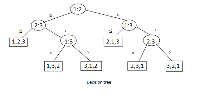
Suppose, We have an input sequence {a₁,a₂...a_n} and assume that all inputs are distinct. We may perform comparison a_i <= a_j & a_i > a_j between two elements a_i and a_j. Here, which pair will make a comparison depends only on the results of the comparisons made so far. For comparison between n elements can be viewed as a binary tree where each node represents a comparison and leaf node gives the permutation of the n elements. This binary tree is also known as the decision tree. A decision tree can be used for any comparison based sorting algorithm.

Here, each internal node label i:j indicates a comparison between a_i and a_j. For any comparison based sorting algorithm, if we ignore detail operation and only consider the comparison between the pair of elements, then the input sequence follows a path in the decision tree from root to leaf.

Lower bound for the worst case

The worst case number of comparison for comparison based sorting algorithm is equal to the longest path of the decision tree from the root. Let's consider a decision tree of height h with l reachable leaves. There are n inputs with n! possible outputs. Each of the permutations of n elements appears on leaves. A binary tree of height h has maximum 2^h leaves. Path having the maximum height represents the worst case. But decision tree might not be a complete binary tree so it can have less than 2^h leaves.
n! <= l <= 2^h

log(n!) = log(1) + log(2) + ... +log(n/2) + ... + log(n)
log(1) + ... +log(n/2) + ... + log(n) >= log(n/2) + log(n/2 + 1) + ... + log(n)
                                      >= log(n/2) + log(n/2) + ... + log(n/2)
                                      >= (n/2)*log(n/2)
                                       = nlogn

By taking logarithms,
h >= log(n!)
= Ω(nlogn)

The lower bound for the worst case analysis is Ω(nlogn). This bound is asymptotically tight.

Lower bound for the average case

Suppose, we have n distinct elements. So, the decision tree has at least n! leaves and each comparison will give either aiaj. If the tree is completely balanced then each leaf's depth is ⌊log₂n!⌋ or ⌈log₂n!⌉. Let's consider D is a decision tree and H(D,l) is the sum of heights for all l leaves.

H(l) represents the minimum sum of heights.

Decision tree D contains two subtree. Let, Number of leaves in the each subtree is m₁ & m₂, respectively.
m₁, m₂ < l
m₁ + m₂ = l & m₁ = m₂ = l/2
H(D,l) = l + H(D1,m₁) + H(D2,m₂)
H(l) = l + min {H(m₁) + H(m₂)}
By the assumption of induction hypothesis:
H(l) <= l + min{m₁logm₁ + m₂logm₂}
H(l) <= l + (l/2)log(l/2) + (l/2)log(l/2)
Average height of the decision tree is -
H(n!) / n! <= log(n!)
= nlogn

The lower bound for the average case analysis is Ω(nlogn).

Lower bound for randomized algorithms

Let, a randomized algorithm A as a probability distribution over deterministic algorithms.

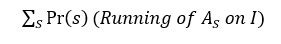
The running time of the randomized algorithm is a random variable and the sequences S correspond to the elementary events. The probability distribution over all the deterministic algorithms is A_S. On some input I, the expected number of comparisons made by randomized algorithm A is -

The expected running time of the randomized algorithm is equal to the average over deterministic algorithms. The running time of the deterministic algorithm is ⌊log₂n!⌋. Average case running time of the randomized algorithm is -

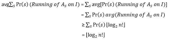
Any randomized comparison based sorting also takes Ω(nlogn) steps.

Bound for non-comparison based sorting

Counting sort, radix sort, bucket sort are known as non-comparison based sorting. These algorithms make no comparison. These are also known as linear sorting algorithms. They don't need a comparison decision tree.

Counting sort uses the key values for sorting, where N is the number of inputs and K is the maximum element. Counting sort takes O(N+K) time which is better than comparison based sorting. If N is as large as K then this is O(N). Since non-comparison-based sorting algorithms don't make a comparison, it allows sorting at linear time.

References

• Lecture 5 on "Lower bounds for sorting" by Avrim Blum, Professor at Carnegie Mellon University (CMU): PDF on cmu.edu